Download
1 / 53
560 likes | 733 Vues
Continental lithosphere investigations using seismological tools. Seismology- lecture 5 Barbara Romanowicz, UC Berkeley. CIDER2012, KITP. Seismological tools. Seismic tomography: surface waves, overtones Volumetric distribution of heterogeneity “smooth” structure – depth resolution ~50 km

E N D
Continental lithosphere investigations using seismological tools Seismology- lecture 5 Barbara Romanowicz, UC Berkeley CIDER2012, KITP
Seismological tools • Seismic tomography: surface waves, overtones • Volumetric distribution of heterogeneity • “smooth” structure – depth resolution ~50 km • Overtones important for the study of continental lithosphere • Additional constraints from anisotropy • “Receiver functions” • Detection of sharp boundaries (i.e. Moho, LAB?, MLD?) • “Long range seismic profiles” – • Several 1000 km long • Map sharp boundaries/regions of strong scattering • “Shear wave splitting” analysis • Teleseismic P and S wave travel times: constraints on average velocities across the upper mantle
ArcheanCratons • Stable regions of continents, relatively undeformed since Precambrian • Structure and formation of the cratonic lithosphere • How did they form? • How did they remain stable since the archean time? • How thick is the cratonic lithosphere? • What is its thermal structure and composition?
Upper mantle under cratons Strength Transitional layer Transitional layer From heat flow Data ~200 km Cooper et al., 2004; Lee, 2006; Cooper and Conrad, 2009
B A Density Structure In situ densities normative densities 3.35 Mg/m3 3.40 Mg/m3 3.40 Mg/m3 A 3.40 Mg/m3 B A B Isopycnic (Equal-Density) Hypothesis The temperature difference between the cratonictectosphere and the convecting mantle is density-compensated by the depletion of the tectosphere in Fe and Al relative to Mg by the extraction of mafic fluids. Courtesy of Tom Jordan
How thick is the cratonic lithosphere? • Jordan (1975,1978) “tectosphere” ~400 km • Heat flow data, magnetotelluric, xenoliths ~200 km (e.g. Mareschal and Jaupart, 2004; Carlson et al., 2005; Jones et al., 2003) • Receiver functions (Rychert and Shearer, 2009): ~ 100 km?
Cluster analysis of upper mantle structure from seismic tomography Isotropic Vs S362ANI SEMum Lekic and Romanowicz, EPSL, 2011
N=2 Clustering analysis of SEMum model N=3 N=6 N=4 N=5 Lekic and Romanowicz 2011,EPSL
3D temperature variations based on inversion of long period seismic waveforms (purely thermal interpretation) Cammarano and Romanowicz, PNAS, 2007
Continental geotherms obtained with a purely thermal interpretation are too cold => compositional signature modified from Mareschal et al., 2004 Courtesy of F. Cammarano, 2008
From global S wave tomography: cratonic lithosphere is thick and fast Kustowski et al., 2008 Cammarano and Romanowicz, 2007
Rayleigh waveovertones By including overtones, we can see into the transition zone and the top of the lower mantle. after Ritsema et al, 2004
P Receiver functions: P-RF P-RF Ray Paths Converted phase: PdS Reading EPSL 2006
Depth of “LAB” from receiver function analysis Rychert and Shearer, Science, 2009
Seismic anisotropy • In an anisotropic structure, seismic waves propagate with different velocities in different directions. • The main causes of anisotropy are: • SPO (shape-Preferred Orientation) • LPO (lattice-preferred orientation)
Seismic anisotropy • In the presence of flow, anisotropic crystals will tend to align in a particular direction, causing seismic anisotropy at a macroscopic level. • In the earth, anisotropy is found primarily: • in the upper mantle (olivine+ deformation) • in the lowermost mantle (D” region) • in the inner core (iron crystals)
Wave propagation in an elastic medium -------------------- Linear relationship between strain and stress: i,j,k ->1,2,3 Strain tensor Stress tensor ui: displacement Elastic tensor : 4-th order tensor which characterizes the medium In the most general case the elastic tensor has 21 independent elements
Special case 1: Isotropic medium : m = shear modulus Compressional modulus l,m: Lamé parameters
Types of anisotropy • General anisotropic model: 21 independent elements of the elastic tensor Cijkl • Surface waves (and overtones) are sensitive to a subset, (13 to 1st order), of which only a small number can be resolved: • Radial anisotropy (5 parameters)- VTI • Azimuthal anisotropy (8 parameters)
Radial Anisotropy (or transverse isotropy) • e.g. SPO: • Anisotropy due to layering • Radial anisotropy • 5 independent elements • of the elastic tensor:A,C,F,L,N (Love, 1911) • L = ρ Vsv2 • N = ρ Vsh2 • C = ρVpv2 • A = ρ Vph2 • = F/(A-2L)
Anisotropy in the upper mantle Azimuthal dependence of seismic wave velocities supports the idea that there is lattice preferred orientation in the Pacific lithosphere associated with the shear caused by plate motion. (Hess, 1964) Fast direction of olivine: [100] aligns with spreading direction Spreading direction Pn wave velocities in Hawaii, where azimuth zero is 90o from the spreading direction Pn is a P wave which propagates right below the Moho.
(A, C, F, L, N, B1,2, G1,2, H1,2, E1,2) Azimuthal anisotropy: • Velocity depends on the direction of propagation in the horizontal plane Where y is the azimuth counted counterclockwise from North a,b,c,d,e are combinations of 13 elements of elastic tensor Cijkl
(A, C, F, L, N, B1,2, G1,2, H1,2, E1,2) (A0, C0, F0, L0, N0, , ) x y Axis of symmetry z Vectorialtomography (Montagner and Nataf, 1988) Orthotropic medium: hexagonal symmetry with inclined symmetry axis (L0, N0, , ) Use lab. measurements of mantle rocks to establish proportionalities between P and S anisotropies (A,C / L, N), and ignore some azimuthal terms
Isotropic velocity Radial Anisotropy x = (Vsh/Vsv)2 Azimuthal anisotropy Hypothetical convection cell Montagner, 2002
Depth = 140 km “SH”: horizontally polarized S waves “SV”: vertically polarized S waves “hybrid”: both
Depth= 100 km Pacific ocean radial anisotropy: Vsh > Vsv Ekstrom and Dziewonski, 1997 Montagner, 2002
Surface wave anisotropy Ekström et al., 1997 Dispersion of Rayleigh waves with 60 second period (most sensitive to depths of about 80-100 km. Orange is slow, blue is fast. Red lines show the fast axis of anisotropy.
Predictions from surface wave inversion SKS splitting measurements Montagner et al. 2000
SKS splitting observations In an isotropic medium, SKS should be polarized as “SV” and observed on the radial component, but NOT on the transverse component
SKS Splitting Observations Interpreted in terms of a model of a layer of anisotropy with a horizontal symmetry axis Dt = time shift between fast and slow waves Yo = Direction of fast velocity axis Montagner et al. (2000) show how to relate surface wave anisotropy and shear wave splitting Huang et al., 2000
Station averaged SKS splitting is robust And expresses the integrated effect of anisotropy over the depth of the upper mantle Wolfe and Silver, 1998
Surface waves + overtones + SKS splitting Absolute Plate Motion Marone and Romanowicz, 2007
Couette Flow Channel Flow Absolute Plate Motion From Turcotte and Schubert, 1982
Continuous lines: % Fo (Mg) from Griffin et al. 2004 Grey: Fo%93 black: Fo%92 Yuan and Romanowicz, Nature, 2010
YKW3 ULM Change In direction with depth Fast axis direction Isotropic Vs Azimuthal anisotropy strength
A Geodynamical modeling: Estimation of thermal layer thickness from chemical thickness From : Cooper et al. 2004 A’ Yuan and Romanowicz, Nature, 2010
LAB in the western US and MLD in the craton occur at nearly same depth LAB MLD Receiver functions
LAB: top of asthenosphere • MLD: in the middle of high Vs lid, also detected with azimuthal anistropy MLD LAB
Long range seismic profiles 8o discontinuity Thybo and Perchuc, 1997
Isotropic velocity North America Azimuthal anisotropy North American continent Yuan et al., 2011
100 to 140 km Less depleted Root x 200 to 250 km: LAB
Does this hold on other cratons? • At least in some…
Arabian Shield Anisotropic MLD from Receiver functions Levin and Park, 2000,
Need to combine information: • Long period seismic waves (isotropic and anisotropic) • Receiver functions • SKS splitting