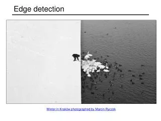
Edge Detection

1. Edge Detection

2. Edge detection • Convert a 2D image into a set of curves • Extracts salient features of the scene • More compact than pixels

3. Origin of Edges • Edges are caused by a variety of factors surface normal discontinuity depth discontinuity surface color discontinuity illumination discontinuity

4. Edge detection • How can you tell that a pixel is on an edge?

5. Profiles of image intensity edges

6. Edge detection • Detection of short linear edge segments (edgels) • Aggregation of edgels into extended edges • (maybe parametric description)

7. Edgel detection • Difference operators • Parametric-model matchers

8. Edge is Where Change Occurs • Change is measured by derivative in 1D • Biggest change, derivative has maximum magnitude • Or 2nd derivative is zero.

9. The gradient direction is given by: • how does this relate to the direction of the edge? • The edge strength is given by the gradient magnitude Image gradient • The gradient of an image: • The gradient points in the direction of most rapid change in intensity

10. The discrete gradient • How can we differentiate a digital image f[x,y]? • Option 1: reconstruct a continuous image, then take gradient • Option 2: take discrete derivative (finite difference) How would you implement this as a cross-correlation?

11. The Sobel operator • Better approximations of the derivatives exist • The Sobel operators below are very commonly used • The standard defn. of the Sobel operator omits the 1/8 term • doesn’t make a difference for edge detection • the 1/8 term is needed to get the right gradient value, however

12. Gradient operators (a): Roberts’ cross operator (b): 3x3 Prewitt operator (c): Sobel operator (d) 4x4 Prewitt operator

13. Effects of noise • Consider a single row or column of the image • Plotting intensity as a function of position gives a signal Where is the edge?

14. Look for peaks in Solution: smooth first Where is the edge?

15. Derivative theorem of convolution • This saves us one operation:

16. Laplacian of Gaussian • Consider Laplacian of Gaussian operator Where is the edge? Zero-crossings of bottom graph

17. 2D edge detection filters • is the Laplacian operator: Laplacian of Gaussian Gaussian derivative of Gaussian

18. Optimal Edge Detection: Canny • Assume: • Linear filtering • Additive iid Gaussian noise • Edge detector should have: • Good Detection. Filter responds to edge, not noise. • Good Localization: detected edge near true edge. • Single Response: one per edge.

19. Optimal Edge Detection: Canny (continued) • Optimal Detector is approximately Derivative of Gaussian. • Detection/Localization trade-off • More smoothing improves detection • And hurts localization. • This is what you might guess from (detect change) + (remove noise)

20. The Canny edge detector • original image (Lena)

21. The Canny edge detector norm of the gradient

22. The Canny edge detector thresholding

23. The Canny edge detector thinning (non-maximum suppression)

24. Non-maximum suppression • Check if pixel is local maximum along gradient direction • requires checking interpolated pixels p and r

25. Predicting the next edge point Assume the marked point is an edge point. Then we construct the tangent to the edge curve (which is normal to the gradient at that point) and use this to predict the next points (here either r or s). (Forsyth & Ponce)

26. Hysteresis • Check that maximum value of gradient value is sufficiently large • drop-outs? use hysteresis • use a high threshold to start edge curves and a low threshold to continue them.

27. Effect of  (Gaussian kernel size) original Canny with Canny with • The choice of depends on desired behavior • large detects large scale edges • small detects fine features

28. Scale • Smoothing • Eliminates noise edges. • Makes edges smoother. • Removes fine detail. (Forsyth & Ponce)

30. fine scale high threshold

31. coarse scale, high threshold

32. coarse scale low threshold

33. first derivative peaks Scale space (Witkin 83) • Properties of scale space (w/ Gaussian smoothing) • edge position may shift with increasing scale () • two edges may merge with increasing scale • an edge may not split into two with increasing scale larger Gaussian filtered signal

34. Edge detection by subtraction original

35. Edge detection by subtraction smoothed (5x5 Gaussian)

36. Edge detection by subtraction Why does this work? smoothed – original (scaled by 4, offset +128) filter demo

37. Gaussian - image filter Gaussian delta function Laplacian of Gaussian

38. An edge is not a line... How can we detect lines ?

39. Finding lines in an image • Option 1: • Search for the line at every possible position/orientation • What is the cost of this operation? • Option 2: • Use a voting scheme: Hough transform

40. Finding lines in an image • Connection between image (x,y) and Hough (m,b) spaces • A line in the image corresponds to a point in Hough space • To go from image space to Hough space: • given a set of points (x,y), find all (m,b) such that y = mx + b y b b0 m0 x m image space Hough space

41. A: the solutions of b = -x0m + y0 • this is a line in Hough space Finding lines in an image • Connection between image (x,y) and Hough (m,b) spaces • A line in the image corresponds to a point in Hough space • To go from image space to Hough space: • given a set of points (x,y), find all (m,b) such that y = mx + b • What does a point (x0, y0) in the image space map to? y b y0 x0 x m image space Hough space

42. Hough transform algorithm • Typically use a different parameterization • d is the perpendicular distance from the line to the origin •  is the angle this perpendicular makes with the x axis • Why?

43. Hough transform algorithm • Typically use a different parameterization • d is the perpendicular distance from the line to the origin •  is the angle this perpendicular makes with the x axis • Why? • Basic Hough transform algorithm • Initialize H[d, ]=0 • for each edge point I[x,y] in the image for  = 0 to 180 H[d, ] += 1 • Find the value(s) of (d, ) where H[d, ] is maximum • The detected line in the image is given by • What’s the running time (measured in # votes)?

44. Extensions • Extension 1: Use the image gradient • same • for each edge point I[x,y] in the image compute unique (d, ) based on image gradient at (x,y) H[d, ] += 1 • same • same • What’s the running time measured in votes? • Extension 2 • give more votes for stronger edges • Extension 3 • change the sampling of (d, ) to give more/less resolution • Extension 4 • The same procedure can be used with circles, squares, or any other shape

45. Extensions • Extension 1: Use the image gradient • same • for each edge point I[x,y] in the image compute unique (d, ) based on image gradient at (x,y) H[d, ] += 1 • same • same • What’s the running time measured in votes? • Extension 2 • give more votes for stronger edges • Extension 3 • change the sampling of (d, ) to give more/less resolution • Extension 4 • The same procedure can be used with circles, squares, or any other shape

46. Hough demos Line : http://www/dai.ed.ac.uk/HIPR2/houghdemo.html http://www.dis.uniroma1.it/~iocchi/slides/icra2001/java/hough.html Circle : http://www.markschulze.net/java/hough/

47. Hough Transform for Curves • The H.T. can be generalized to detect any curve that can be expressed in parametric form: • Y = f(x, a1,a2,…ap) • a1, a2, … ap are the parameters • The parameter space is p-dimensional • The accumulating array is LARGE!

48. Corners contain more edges than lines. Corner detection • A point on a line is hard to match.

49. Corners contain more edges than lines. • A corner is easier

50. Edge Detectors Tend to Fail at Corners