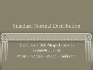
The standard normal distribution
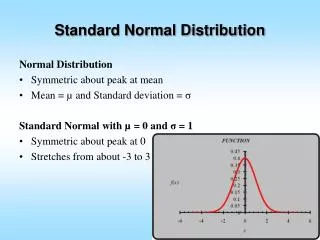
a.k.a. “bell curve”. The standard normal distribution. The normal distribution. If a characteristic is normally distributed in a population, the distribution of scores measuring that characteristic will form a bell-shaped curve.


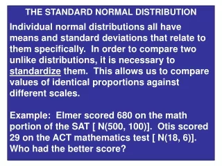
The standard normal distribution
E N D
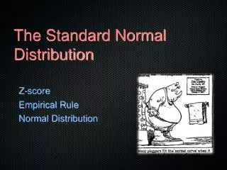
Presentation Transcript
a.k.a. “bell curve” The standard normal distribution
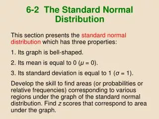
The normal distribution • If a characteristic is normally distributed in a population, the distribution of scores measuring that characteristic will form a bell-shaped curve. • This assumes every member of the population possesses some of the characteristic, though in differing degrees. • examples: height, intelligence, self esteem, blood pressure, marital satisfaction, etc. • Researchers presume that scores on most variables are distributed in a “normal” fashion, unless shown to be otherwise • Including communication variables
The normal distribution • Only interval or ratio level data can be graphed as a distribution of scores: • Examples: physiological measures, ratings on a scale, height, weight, age, etc. • Any data that can be plotted on a histogram • Nominal and ordinal level data cannot be graphed to show a distribution of scores • nominal data is usually shown on a frequency table, pie chart, or bar chart
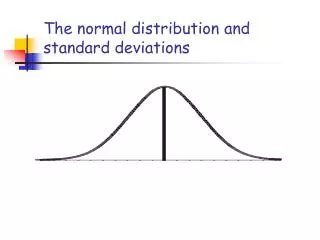
More about the normal distribution • Lower scores are found toward the left-hand side of the curve. • Medium scores occupy the middle portion of the curve • this is where most scores congregate, since more people are average or typical than not • Higher scores are found toward the right-hand side of the curve • In theory, the “tails” of the curve extend to infinity (e.g. asymptotic) lower scores medium scores higher scores
More about the normal distribution mean median mode • In a normal distribution, the center point is the exact middle of the distribution (the “balance point”) • In a normal, symmetrical distribution, the mean, median, and mode all occupy the same place
Comparing groups based on their means and standard deviations • Note the height of the curve does not reflect the size of the mean, but rather the number of scores congregated about the mean
Non-normal distributions • Kurtosis refers to how “flat” or “peaked” a distribution is. • In a “flat” distribution scores are spread out farther from the mean • There is more variability in scores, and a higher standard deviation • In a “peaked” distribution scores are bunched closer to the mean • There is less variability in scores, and a lower standard deviation kurtosis
kurtosis • Non-normal distributions may be: • Leptokurtic (or peaked) • Scores are clustered closer to the mean • Mesokurtic (normal, bell shaped) • Platykurtic (flat) • Scored are spread out farther from the mean
Non-normal distributions • Skewness refers to how nonsymmetrical or “lop-sided” a distribution is. • If the tail extends toward the right, a distribution is positively skewed • If the tail extends toward the left, a distribution is negatively skewed skewness
More abut skewness • In a positively skewed distribution, the mean is larger than the median • In a negatively skewed distribution, the mean is smaller than the median • Thus, if you know the mean and median of a distribution, you can tell if it is skewed, and “guesstimate” how much.
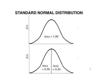
Standard deviations and the normal distribution • Statisticians have calculated the proportion of the scores that fall into any specific region of the curve • For instance, 50% of the scores are at or below the mean, and 50% of the scores are at or above the mean 50% 50%
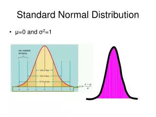
Standard deviations and the normal curve 68.26% • Statisticians have designated different regions of the curve, based on the number of standard deviations from the mean • Each standard deviation represents a different proportion of the total area under the curve • Most scores or observations (approx. 68%) fall within +/- one standard deviation from the mean 34.13% 34.13% -3 SD -2 SD -1 SD +1 SD +2 SD +3 SD
Standard deviations and the normal curve • Thus, the odds of a particular score, or set of scores, falling within a particular region are equal to the percentage of the total area occupied by that region 34.13% 34.13% 13.59% 13.59% 2.14% 2.14% -3 SD -2 SD -1 SD +1 SD +2 SD +3 SD 68.26% 95.44% 99.72%%
Probability theory and statistical significance random score • The odds that a score or measurement taken at random will fall in a specific region of the curve are the same as the percentage of the area represented by that region. • Example: The odds that a score taken at random will fall in the red area are roughly 68%. -3 -2 +1 +1 +2 +3 68.26%
Probability theory and statistical significance • The probability of a random or chance event happening in any specific region of the curve is also equal to the percentage of the total area represented by that region • the odds of a chance event happening two standard deviations beyond the mean are approximately 4.28%, or less than 5% -3 -2 +1 +1 +2 +3 The odds of a random or chance event happening in this region are 2.14% The odds of a random or chance event happening in this region are 2.14%
Probability theory and statistical significance • When a researcher states that his/her results are significant at the p < .05 level, the researcher means the results depart so much from what would be expected by chance that he/she is 95% confident they could not have been obtained by chance alone. • The results are probably due to the experimental manipulation, and not due to chance -2 -1 +1 +2 -3 +3 By chance alone, results should wind up in either of these two regions less than 5% of the time
Probability theory and statistical significance • When a researcher states that his/her results are significant at the p < .01 level, the researcher means the results depart so much from what would be expected by chance alone, that he/she is 99% confident they could not have been obtained merely by chance. • The results are probably due to the experimental manipulation and not to chance -2 -1 +1 +2 -3 +3 By chance alone, results should wind up in either of these two regions less than 1% of the time.
Probability theory and statistical significance • When a researcher employs a nondirectional hypothesis, the researcher is expecting a significant difference at either “tail” of the curve. • When a researcher employs a directional hypothesis, the researcher expects a significant difference at one specific “tail” of the curve. -2 -1 +1 +2 -3 +3 Nondirectional hypothesis either tail of the curve Directional hypothesis one tail or the other
Probability theory and statistical significance • The “control” group in an experiment represents normalcy. • Scores for a “control” group are expected to be typical, or “average.” • The “treatment” group in an experiment is exposed to a manipulation or stimulus condition. • Scores for a “treatment” group are expected to be significantly different from those of the control group. • The researcher expects the “treatment” group to be 2 std. dev. beyond the mean of the control group. -2 -1 +1 +2 -3 +3 The control group should be in the middle of the distribution The treatment group is expected to be 2 std. dev beyond the mean