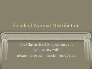
The Standard Normal Distribution
140 likes | 289 Vues
The Standard Normal Distribution. Section 2.2.1. Starter. Weights of adult male Norwegian Elkhounds are N(42, 2) pounds. What weight would represent the 16 th percentile?. Today’s Objectives. State mean and standard deviation for The Standard Normal Distribution.

The Standard Normal Distribution
E N D
Presentation Transcript
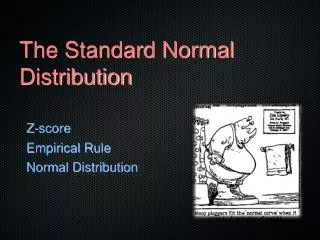
The Standard Normal Distribution Section 2.2.1
Starter • Weights of adult male Norwegian Elkhounds are N(42, 2) pounds. • What weight would represent the 16th percentile?
Today’s Objectives • State mean and standard deviation for The Standard Normal Distribution. • Given a raw score from a normal distribution, find the standardized “z-score”. • Use the Table of Standard Normal Probabilities to find: • the area between given borders of the Standard Normal curve. • The raw score (x value) that leads to a given area.
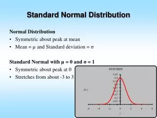
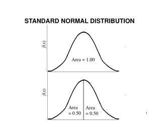
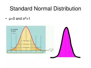
Standardizing Observations • All normal distributions have fundamentally the same shape. • If we measure the x axis in units of size σ about a center of 0, then they are all exactly the same curve. • This is called the Standard Normal Curve • To standardize observations, we change from x values (the raw observations) to z values (the standardized observations) by the formula:
The Standard Normal Distribution • Notice that the z-score formula always subtracts μ from each observation. • So the mean is always shifted to zero • Also notice that the shifted values are divided by σ, the standard deviation. • So the units along the z-axis represent numbers of standard deviations • Thus the Standard Normal Distribution is always N(0,1).
Example 2.3 (p 84) • The heights of young women are: N(64.5, 2.5) • Use the formula to find the z-score of a woman 68 inches tall. • A woman’s standardized height is the number of standard deviations by which her height differs from the mean height of all young women.
Normal Distribution Calculations • What proportion of all young women are less than 68 inches tall? (Examples 2.4 & 2.5, p 86) • Notice that this does not fall conveniently on one of the σ borders, so the empirical rule does not help! • We already found that 68 inches corresponds to a z-score of 1.4 • So what proportion of all standardized observations fall to the left of z = 1.4? • Since the area under the Standard Normal Curve is always 1, we can ask instead what is the area under the curve and to the left of z=1.4 • For that, we need a table.
The Standard Normal Table • Find Table A on pages 13 & 14 of the handout • It is also in your textbook inside the front cover • Z-scores (to the nearest tenth) are in the left column • The other 10 columns round z to the nearest hundredth • Find z = 1.4 in the table and read the area • You should find area to the left = .9192 • So the proportion of observations less than z = 1.4 is about 92% • Now put the answer in context: “About 92% of all young women are 68 inches tall or less.”
What about area above a value? • Still using the N(64.5, 2.5) distribution, what proportion of young women have a height of 61.5 inches or taller? • Z = (61.5 – 64.5)/2.5 = -1.2 • From Table A, area to the left of -1.2 =.1151 • So area to the right = 1 - .1151 = .8849 • So about 88% of young women are 61.5” tall or taller.
What about area between two values? • What proportion of young women are between 61.5” and 68” tall? • We already know 68” gives z = 1.4 and area to the left of .9192 • We also know 61.5” gives z = -1.2 and area to the left of .1151 • So just subtract: .9192 - .1151 = .8041 • So about 80% of young women are between 61.5” and 68” tall • Remember to write your answer IN CONTEXT!!!
Given a proportion, find the observation x (Ex. 2.8, p 90) • SAT Verbal scores are N(505, 110). How high must you score to be in the top 10%? • If you are in the top 10%, there must be 90% below you (to the left). • Find .90 (or close to it) in the body of Table A. What is the z-score? • You should have found z = 1.28 • Now solve the z definition equation for x • So you need a score of at least 646 to be in the top 10%.
Today’s Objectives • State mean and standard deviation for The Standard Normal Distribution. • Given a raw score from a normal distribution, find the standardized “z-score”. • Use the Table of Standard Normal Probabilities to find: • the area between given borders of the Standard Normal curve. • The raw score (x value) that leads to a given area.
Homework • Read pages 83 – 91 • Do problems 22 – 25