Applying the Standard Normal Distribution to Problems
390 likes | 558 Vues
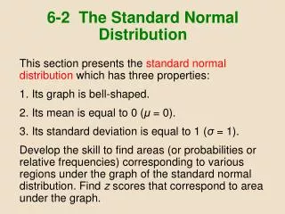
Applying the Standard Normal Distribution to Problems. Real stuff and real numbers in the world of x, z, and Area. Review. Following: a quick review of the Standard Normal Distribution Recall We can find area to the left of some z We can find area to the right of some z

Applying the Standard Normal Distribution to Problems
E N D
Presentation Transcript
Applying the Standard Normal Distribution to Problems Real stuff and real numbers in the world of x, z, and Area
Review • Following: a quick review of the Standard Normal Distribution • Recall • We can find area to the left of some z • We can find area to the right of some z • We can find area between two z values • What’s going to be new here: • Take x problems (real-life) and change them to z problems (Standard Normal Distribution)
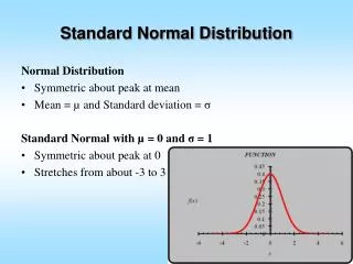
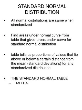
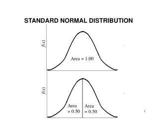
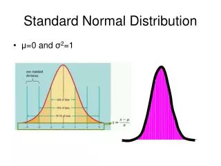
The Standard Normal Distribution is our favorite • This one is the most special of all of them • The mean: • The standard deviation: • Horizontal • Total area between curve and axis = 1.000
Normal Distribution Properties Bluman, Chapter 6
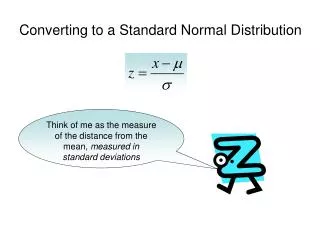
z value (Standard Value) The z value is the number of standard deviations that a particular X value is away from the mean. The formula for finding the z value is: Bluman, Chapter 6
x value Going the other way: If you know the z value and you need to find the x value, 6
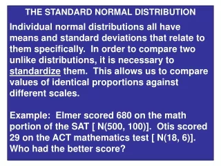
6.2 Applications of the Normal Distributions • The standard normal distribution curve can be used to solve a wide variety of practical problems. The only requirement is that the variable be normally or approximately normally distributed. • For all the problems presented in this chapter, you can assume that the variable is normally or approximately normally distributed. Bluman, Chapter 6
“You can assume that…” • Not every measurement follows the pattern of a bell-shaped a Normal Distribution! • A lot do, so let’s see what we can do with z. • But some are skewed– not normal distribut’n • Some will be uniform – not normal distribut’n • And various others that aren’t normal distrib’n • For those others, today’s methods are Invalid!
Applications of the Normal Distributions • To solve problems by using the standard normal distribution, transform the original variable to a standard normal distribution variable by using the z value formula. • This formula transforms the values of the variable into standard units or z values. Once the variable is transformed, then the Procedure Table and Table E in Appendix C can be used to solve problems. Bluman, Chapter 6
What did that last slide say? • We are given an “x” problem from real life. • The measurements are everyday kinds of units • The values happen to fall in a normal distrib’n. • We change the x problem into a z problem • So it fits a Standard Normal Distribution • Area is Probability and Probability is Area
Example 6-6: Holiday Spending A survey by the National Retail Federation found that women spend on average $146.21 for the Christmas holidays. Assume the standard deviation is $29.44. Find the percentage of women who spend less than $160.00. Assume the variable is normally distributed. Step 1: Draw the normal distribution curve. Bluman, Chapter 6
Example 6-6: Holiday Spending Step 2: Find the z value corresponding to $160.00. Step 3: Find the area to the left of z = 0.47. Table E gives us an area of .6808. 68% of women spend less than $160. Bluman, Chapter 6
The Holiday Spending Example What did they do? Conclusions and Extensions x = $160 Converted to z = 0.47 Area to left is 0.6808 So 68% spend less than $160 Area to right is _______ _____% spend more than $160 • They took an “x” problem • Measurements in dollars • Situation follows a normal distribution (given) • They changed it into a z problem. • Area represented portion of spenders
The Holiday Spending Example Analysis and Printed Table Analysis and TI-84 solution Same assumption Same particular normal dist Same question asked TI-84 can do it all in one step More info next slide > > > • Assumption: Normal distrib • “What % less than $160?” • Converted to • What is area to left of ? • Lookup in printed table • State conclusion: “68%...”
Low x (use -1E99 for “everything to the left”) • Approximates “negative infinity” by • 2ND COMMA (EE) for the “E”, • -99 worked for z problemsbut need better here • High x (use 1E99 for “everything to the right”) • Approximate “positive infinity” by • Mean of the population • Standard deviation of the population
We can input it as an x problem • Under the hood • The TI-84 converts it to a z problem • But it needed to know the mean and standard deviation • When we omit the mean and standard deviation, the TI-84 assumes we are talking z language • You still need to draw pictures and understand concepts and be able to do it “primitively”
Example 6-8: Emergency Response The American Automobile Association reports that the average time it takes to respond to an emergency call is 25 minutes. Assume the variable is approximately normally distributed and the standard deviation is 4.5 minutes. If 80 calls are randomly selected, approximately how many will be responded to in less than 15 minutes? (Added non-Bluman content) • FIRST find the proportion (or percent) that are under 15 minutes response time • THEN multiply the 80 calls by that proportion. Bluman, Chapter 6
Example 6-8: Emergency Response The American Automobile Association reports that the average time it takes to respond to an emergency call is 25 minutes. Assume the variable is approximately normally distributed and the standard deviation is 4.5 minutes. If 80 calls are randomly selected, approximately how many will be responded to in less than 15 minutes? Step 1: Draw the normal distribution curve. Bluman, Chapter 6
Example 6-8: Emergency Response Step 2: Find the z value for 15. Step 3: Find the area to the left of z = -2.22. It is 0.0132. Step 4: To find how many calls will be made in less than 15 minutes, multiply the sample size 80 by 0.0132 to get 1.056. Hence, approximately 1 call will be responded to in under 15 minutes. Bluman, Chapter 6
TI-84 for Emergency Response • Find the proportion using normalcdf(low x, high x, mean, stdev) • Since this is an area, or probability, the result is between 0.0000 and 1.0000 • To scale it up to n=80, multiply by 80 • 2ND ANS recalls the normalcdf() result
More Emergency Response Practice • What percent of calls have response time >25 minutes? • What percent have response time >30 minutes? • What percent have response time between 15 and 30 minutes? • If 3185 calls occur in a month, how many take more than 30 minutes to get a response?
Example 6-7a: Newspaper Recycling Each month, an American household generates an average of 28 pounds of newspaper for garbage or recycling. Assume the standard deviation is 2 pounds. If a household is selected at random, find the probability of its generating between 27 and 31 pounds per month. Assume the variable is approximately normally distributed. Step 1: Draw the normal distribution curve. Bluman, Chapter 6
Example 6-7a: Newspaper Recycling Step 2: Find z values corresponding to 27 and 31. Step 3: Find the area between z = -0.5 and z = 1.5. Table E gives us an area of .9332 - .3085 = .6247. The probability is 62%. Bluman, Chapter 6
Newspaper Recycling, TI-84 • Low x = 27 • High x = 31 • Mean x = 28 • Standard deviation of x = 2
Backwards x problems • They give a proportion or percent of interest • “What x value separates out the low/middle/high %?” • Think: proportions are areas • DRAW A PICTURE • Find the z value and then convert it to an x value.
Example 6-9: Police Academy To qualify for a police academy, candidates must score in the top 10% on a general abilities test. The test has a mean of 200 and a standard deviation of 20. Find the lowest possible score to qualify. Assume the test scores are normally distributed. Step 1: Draw the normal distribution curve. Bluman, Chapter 6
Police Academy (Added guidance not given by Bluman) • You have an area and a nice picture. • Solve the z problem first. What z score separates the top 10% • This is same as “What z separates the bottom 90% (0.9000)?” • When you find the z, convert it to an x answer.
Example 6-9: Police Academy Step 2: Subtract 1 - 0.1000 to find area to the left, 0.9000. Look for the closest value to that in Table E. Step 3: Find X. The cutoff, the lowest possible score to qualify, is 226. Bluman, Chapter 6
TI-84 for Police Academy • Use 2nd DISTR invNorm(area to left, x mean, x stdev) • Area to left = the area (proportion) to the left • Mean of the distribution in x language • Standard deviation of the distribution in x
Example 6-10: Systolic Blood Pressure For a medical study, a researcher wishes to select people in the middle 60% of the population based on blood pressure. If the mean systolic blood pressure is 120 and the standard deviation is 8, find the upper and lower readings that would qualify people to participate in the study. Step 1: Draw the normal distribution curve. Bluman, Chapter 6
Example 6-10: Systolic Blood Pressure Area to the left of the positive z: 0.5000 + 0.3000 = 0.8000. Using Table E, z 0.84. Area to the left of the negative z: 0.5000 – 0.3000 = 0.2000. Using Table E, z - 0.84. The middle 60% of readings are between 113 and 127. X = 120 + 0.84(8) = 126.72 X = 120 - 0.84(8) = 113.28 Bluman, Chapter 6
TI-84 for Blood Pressure • You still have to draw the picture!!!!!!!!!!!!!!!! • Left edge has 0.2000 of the area to its left • Right edge has 0.8000 of the area to its left • (the 0.2000 on the left end + 0.6000 between) • Use invNorm twice! • 2ND ENTER shortcutrecalls first entryand just edit a little
More Blood Pressure Practice • What blood pressure readings define the middle 90%? • The middle 95%? • Separate the bottom 1% from everybody else? • Separate the top 1% from everybody else? • The quartiles (25th and 75th percentiles)?
“Is this a normal distribution?” • A dangerous assumption has been used for this entire lesson. • The question is an important question for statisticians in general. • What follows is a glimpse of one little corner of the specialized task of determining whether a distribution is a normal distribution. • It’s kind of advanced, a fringe topic in this lesson, presented mostly for awareness.
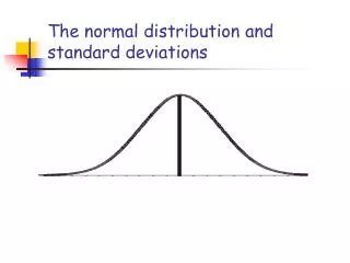
Normal Distributions • A normally shaped or bell-shaped distribution is only one of many shapes that a distribution can assume; however, it is very important since many statistical methods require that the distribution of values (shown in subsequent chapters) be normally or approximately normally shaped. • There are a number of ways statisticians check for normality. We will focus on three of them. Bluman, Chapter 6
Checking for Normality • Histogram • Pearson’s Index PI of Skewness • Outliers • Other Tests • Normal Quantile Plot • Chi-Square Goodness-of-Fit Test • Kolmogorov-Smikirov Test • Lilliefors Test Bluman, Chapter 6
Example 6-11: Technology Inventories A survey of 18 high-technology firms showed the number of days’ inventory they had on hand. Determine if the data are approximately normally distributed. 5 29 34 44 45 63 68 74 74 81 88 91 97 98 113 118 151 158 Method 1: Construct a Histogram. The histogram is approximately bell-shaped. Bluman, Chapter 6
Example 6-11: Technology Inventories Method 2: Check for Skewness. The PI is not greater than 1 or less than 1, so it can be concluded that the distribution is not significantly skewed. Method 3: Check for Outliers. Five-Number Summary: 5 - 45 - 77.5 - 98 - 158 Q1 – 1.5(IQR) = 45 – 1.5(53) = -34.5 Q3 – 1.5(IQR) = 98 + 1.5(53) = 177.5 No data below -34.5 or above 177.5, so no outliers. Bluman, Chapter 6
Example 6-11: Technology Inventories A survey of 18 high-technology firms showed the number of days’ inventory they had on hand. Determine if the data are approximately normally distributed. 5 29 34 44 45 63 68 74 74 81 88 91 97 98 113 118 151 158 Conclusion: • The histogram is approximately bell-shaped. • The data are not significantly skewed. • There are no outliers. Thus, it can be concluded that the distribution is approximately normally distributed. Bluman, Chapter 6