Download
1 / 15
150 likes | 242 Vues
This article examines the progress in climate modeling for the Southern Ocean, focusing on sea ice cover changes and ocean circulation over the last 25 years. It discusses model tests, validations, and trends for AR5 goals and presents weighted averages and analysis of model simulations. The influence of atmospheric circulation, changes in sea ice cover and oceanic circulation over the 21st century are also explored. Additionally, it addresses the method of weighting model results, emphasizing the importance of multidecadal timescales in evaluating models.

E N D
Climate modeling status - goalsPart 2 NOAA photo library
Overview • Main activities since the AR4: • Additional analysis of existing simulations (weighting of models) • Preparation of the models/simulations for AR5 • Model tests and validation in the Southern Ocean: • Tests at the process level • Reproducing the main characteristics of the observed mean state and recent trends.
The sea ice cover over the last 25 years in AR4 models Mean summer and winter ice extent over the period 1981-2000 Shading indicates the % of models that have ice in average over the period 1981-2000 in March (left) and September (right). The analysis is based on 14 models. The observed ice edge is the thick black line. Arzel et al. 2006
The sea ice cover over the last 25 years Trend in ice extent over the period 1981-2000 Arctic (left column) and Antarctic (right column) ice extent and its changes. (a) Mean ice extent. Grey and white shading correspond to minimum and maximum ice extents. (b) Change in annual mean ice extent over the period 1981-2000 and the standard deviation of the ice extent over the same period. Arzel et al. 2006
The sea ice cover over the last 25 years Trend in annual mean ice concentration over the period 1981-2000 Observed annual mean ice concentration trend in % integrated over the period 1979-2004 (left). Same for the average of 16 AOGCMs (right) Lefebvre and Goosse 2008
Influence of atmospheric circulation on the ice concentration Influence of SAM on the sea ice concentration over the last 25 years Regression of the annual mean observed ice concentration (%) with the SAM index over the period 1979-2004 (left). Same for the average of 16 AOGCMs (right) Lefebvre and Goosse 2008
Ocean circulation over the last 25 years Transport trough Drake Passage (Sv) in 12 models Mean Sea also Russell et al., 2006
Changes over the 21st Century Changes in sea ice cover Difference in annual mean ice concentration (%) between the period 2071-2100 and 1979-2004 in scenario SRES-A1B, averaged over 16 models. Lefebvre and Goosse 2008
Changes over the 21st Century Changes in oceanic circulation Difference in annual mean barotropic streamfunction (Sv) between the period 2071-2100 and 1979-2004 in scenario SRES-A1B, averaged over 12 models. Flow is clockwise around a minimum. Lefebvre and Goosse 2008
Weigthed averages Goal: instead of performing simple multimodel average, the results of the various models are weigthed according to some measure of their performance. “The method cannot be fully objective because a number of subjective choices have to be made in applying it.” Conneley and Bacegirdle (2007). Example of method (Conneley and Bacegirdle 2007): Evaluate the Root Mean Square Error for various fields such as mean sea level pressure, height and temperature at 500 hPa ; sea surface temperature, sea ice, surface mass balance over Antarctica, etc. The score (and thus the weight) for each model is deduced from those RMSs.
Weigthed averages Changes in sea ice concentration Difference between weighted and unweighted ensemble mean sea ice concentration projected 21st century change (2080–2099 minus 2004–2023 mean) for (a) DJF, (b) MAM, (c) JJA and (d) SON. Bacegirdle et al. 2008
Analyzing changes over the last 30-50 years Annual mean temperature averaged over the shelf and slope area of the western peninsula in a simulation with the sea-ice-ocean model NEMO-LIM driven by NCEP-NCAR reanalysis. Figure from P. Matthiot
Analyzing changes over the last 30-50 years Anomaly of annual mean sea-ice area (in 106 km2) in the Southern Ocean LOVECLIM with data assimilation Observations (Rayner et al., 2003) The green curve is the estimate based on the HADISST data set ( Rayner et al. 2003). The black line is the averaged over the 6 model simulations while the grey lines are the mean plus and minus one standard deviation of the ensemble. A 11-year running mean has been applied to the time series. The reference period is 1960-2000. Goosse et al., 2009
Analyzing changes over the last 30-50 years Anomaly of annual mean sea-ice area (in 106 km2) in the Southern Ocean LOVECLIM with data assimilation LOVECLIM without data assimilation Ensemble mean of AOGCMs assimilations The black line is the averaged over the 6 model simulations using LOVECLIM with data assimilation. The red line is the mean of an ensemble of 20 simulations made with LOVECLIM but without data assimilation. The blue line is the mean over 16 model simulations performed in the framework of the 4th IPCC report. Goosse et al., 2009
Points to discuss • Could we select a set of key observations/diagnostics to make a benchmark of models in the Southern Ocean ? • (part of the SO climate review article?) • Is there a right way to weight model results? • Insist on multidecadal timescales in the evaluation of models