Download
1 / 28
290 likes | 473 Vues
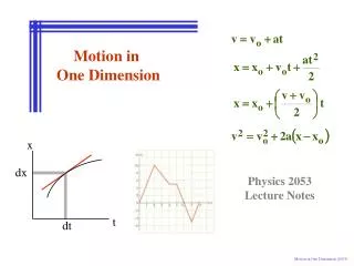
Motion in One Dimension. Displacement. A change in an object’s position: Δx = x f – x i This is a vector quantity Units: m How is displacement different from distance?. Average Velocity and Average Speed.

E N D
Displacement • A change in an object’s position: • Δx = xf – xi • This is a vector quantity • Units: m • How is displacement different from distance?
Average Velocity and Average Speed • Average Velocity: the displacement of an object divided by the time interval over which that displacement occurred • Vector quantity (sign gives direction) • Units: m/s • Average Speed: the total distance traveled divided by the total time interval to travel that distance • Scalar quantity (always positive)
B A Dx Dt Average Velocity from a Graph x t
A x B Dx Dt t Average Velocity from a Graph
Average Acceleration • Average acceleration of an object is the change in that objects velocity divided by the time interval over which that change occurred • This is how fast the velocity is changing over time • You can also think about it as:
B A Dx Dt Average Acceleration from a Graph v t
x t Instantaneous Velocity and Speed A Average Velocity from a graph B Remember that the average velocity between the time at A and the time at B is the slope of the connecting line.
x t Instantaneous Velocity and Speed A B What happens if A and B become closer to each other?
x t Instantaneous Velocity and Speed A B What happens if A and B become closer to each other?
x t Instantaneous Velocity and Speed B A What happens if A and B become closer to each other?
x t Instantaneous Velocity and Speed B A What happens if A and B become closer to each other?
x t Instantaneous Velocity and Speed A and B are effectively the same point. The time difference is effectively zero. B A The line “connecting” A and B is a tangent line to the curve. The velocity at that instant of time is represented by the slope of this tangentline.
Remember that a limit is used to define a derivative by:
Instantaneous Velocity and Speed • Instantaneous velocity is the limiting value of Δx/Δt as Δt approaches zero, or the derivative of x with respect to t: • The instantaneous speed of an object is the magnitude of its velocity
v t Average and Instantaneous Acceleration Instantaneous acceleration is represented by the slope of a tangent to the curve on a v/t graph. A Average acceleration is represented by the slope of a line connecting two points on a v/t graph. C B
Instantaneous acceleration is the limiting value of Δv/Δt as Δt approaches zero, or the derivative of v with respect to t: Instantaneous Acceleration • Acceleration can also be referred to as the second derivative of position with respect to time. • Just don’t let the new notation scare you; think of the d as a baby Δ, indicating a very tiny change!
Now YOU try it! Try these phun problems using the calculus
Derivatives: the graphical representation • Look closely at each of these graphs (all of which are for the same motion) • x vs t, v vs t, and a vs t • Remember that derivatives have to do with slope (over an increasingly small interval) • Analyze each time interval and see if you can understand how these graphs are connected
Now YOU try it! Using your knowledge of how position, velocity, and acceleration are connected, analyze and plot the following graphs
x v a t t t Acceleration vs time Position vs time Velocity vs time Draw representative graphs for a particle which is stationary.
x v a t t t Acceleration vs time Position vs time Velocity vs time Draw representative graphs for a particle which has constant non-zero velocity.
x v a t t t Acceleration vs time Position vs time Velocity vs time Draw representative graphs for a particle which has constant non-zero acceleration.
Given this graph of position vs time, plot the corresponding v vs t and a vs t graphs
Given this graph of velocity vs time, plot the corresponding x vs t and a vs t graphs