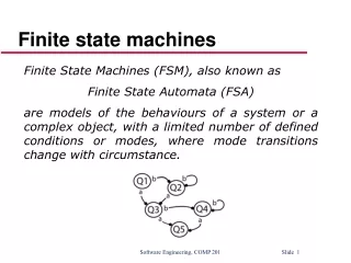
Nondeterministic Finite State Machines
Nondeterministic Finite State Machines. Chapter 5. Nondeterminism. Imagine adding to a programming language the function choice in either of the following forms: 1. choose (action 1;; action 2;; … action n ) 2. choose ( x from S : P ( x )). Implementing Nondeterminism.

Nondeterministic Finite State Machines
E N D
Presentation Transcript
Nondeterministic Finite State Machines Chapter 5
Nondeterminism Imagine adding to a programming language the function choice in either of the following forms: 1. choose (action 1;; action 2;; … action n ) 2. choose(x from S: P(x))
Implementing Nondeterminism before the first choice choose makes first call to choose first call to choose choice 1 choice 2 second call to choose second call to choose choice 1 choice 2
Nondeterminism • What it means/implies • We could guess and our guesses would lead us to the answer correctly (if there is an answer).
Definition of an NDFSM M = (K, , , s, A), where: K is a finite set of states is an alphabet sK is the initial state AK is the set of accepting states, and is the transition relation. It is a finite subset of (K ( {}) ) K state input or empty string state Where you are What you see Where you go Cartesian product
Accepting by an NDFSM M accepts a string w iff there exists some path along which w drives M to some element of A. The language accepted by M, denoted L(M), is the set of all strings accepted by M.
Sources of Nondeterminism What differ from determinism?
Analyzing Nondeterministic FSMs Two approaches: • Explore a search tree: • Follow all paths in parallel
Optional Substrings L = {w {a, b}* : w is made up of an optional a followed by aa followed by zero or more b’s}.
Optional Substrings L = {w {a, b}* : w is made up of an optional a followed by aa followed by zero or more b’s}.
Optional Substrings L = {w {a, b}* : w is made up of an optional a followed by aa followed by zero or more b’s}. M = (K, , , s, A) = ({q0, q1, q2 , q3}, {a, b}, , q0, {q3}), where = {((q0, a), q1), ((q0, ), q1), ((q1, a), q2), ((q2, a), q3), ((q3, b), q3)} How many elements does have?
Multiple Sublanguages L = {w {a, b}* : w = aba or |w| is even}.
Multiple Sublanguages L = {w {a, b}* : w = aba or |w| is even}.
Multiple Sublanguages L = {w {a, b}* : w = aba or |w| is even}.
Multiple Sublanguages L = {w {a, b}* : w = aba or |w| is even}. M = (K, , , s, A) = ({q0, q1, q2, q3, q4, q5, q6}, {a, b}, , q0, {q4, q5}), where = {((q0, ), q1), ((q0, ), q5), ((q1, a), q2), ((q2, b), q3), ((q3, a), q4), ((q5, a), q6), ((q5, b), q6), ((q6, a), q5), ((q6, b), q5)} Do you start to feel the power of nondeterminism?
The Missing Letter Language Let = {a, b, c, d}. Let LMissing= {w : there is a symbol ai not appearing in w} Recall the complexity of DFSM!
Pattern Matching L = {w {a, b, c}* : x, y {a, b, c}* (w = xabcabby)}. A DFSM:
Pattern Matching L = {w {a, b, c}* : x, y {a, b, c}* (w = xabcabby)}. A DFSM: An NDFSM:
Pattern Matching with NDFSMs L = {w {a, b}* : x, y {a, b}* : w = xaabbby or w = xabbaby }
Multiple Keywords L = {w {a, b}* : x, y {a, b}* ((w = xabbaay) (w = xbabay))}.
Checking from the End L = {w {a, b}* : the fourth to the last character is a}
Checking from the End L = {w {a, b}* : the fourth to the last character is a}
Another Pattern Matching Example L = {w {0, 1}* : w is the binary encoding of a positive integer that is divisible by 16 or is odd}
Another NDFSM L1= {w {a, b}*: aa occurs in w} L2= {x {a, b}*: bb occurs in x} L3= {y : L1 or L2 } L4= L1L2 M1 = M2= M3= M4=
Analyzing Nondeterministic FSMs Does this FSM accept: baaba Remember: we just have to find one accepting path.
Analyzing Nondeterministic FSMs Two approaches: • Explore a search tree: • Follow all paths in parallel
Dealing with Transitions eps(q) = {pK : (q, w) |-*M (p, w)}. eps(q) is the closure of {q} under the relation {(p, r) : there is a transition (p, , r) }. How shall we compute eps(q)? It simply means the states reachable without consuming input.
An Algorithm to Compute eps(q) eps(q: state) = result = {q}. While there exists some presult and some rresult and some transition (p, , r) do: Insert r into result. Return result.
An Example of eps eps(q0) = eps(q1) = eps(q2) = eps(q3) =
Simulating a NDFSM ndfsmsimulate(M: NDFSM, w: string) = • current-state = eps(s). • While any input symbols in w remain to be read do: • c = get-next-symbol(w). • next-state = . • For each state q in current-state do: For each state p such that (q, c, p) do: next-state = next-stateeps(p). • current-state = next-state. • If current-state contains any states in A, accept. Else reject.
Nondeterministic and Deterministic FSMs Clearly: {Languages accepted by a DFSM} {Languages accepted by a NDFSM} More interestingly: Theorem: For each NDFSM, there is an equivalent DFSM.
Nondeterministic and Deterministic FSMs Theorem: For each NDFSM, there is an equivalent DFSM. Proof: By construction: Given a NDFSM M = (K, , , s, A), we construct M' = (K', , ', s', A'), where K' = P(K) s' = eps(s) A' = {QK : QA} '(Q, a) = {eps(p): pK and (q, a, p) for some qQ} May create many unreachable states
An Algorithm for Constructing the Deterministic FSM 1. Compute the eps(q)’s. 2. Compute s' = eps(s). 3. Compute ‘. 4. Compute K' = a subset of P(K). 5. Compute A' = {QK' : QA}. • The algorithm • Proves NDFSM DFSM • Allows us to solve problems using NDFSM then construct equivalent DFSM
The Algorithm ndfsmtodfsm • ndfsmtodfsm(M: NDFSM) = • 1. For each state q in KM do: • 1.1 Compute eps(q). • 2. s' = eps(s) • 3. Compute ': • 3.1 active-states = {s'}. • 3.2 ' = . • 3.3 While there exists some element Q of active-states for • which ' has not yet been computed do: • For each character c in M do: • new-state = . • For each state q in Q do: • For each state p such that (q, c, p) do: • new-state = new-stateeps(p). • Add the transition (Q, c, new-state) to '. • If new-stateactive-states then insert it. • 4. K' = active-states. • 5. A' = {QK' : QA }.
An Example – Optional Substrings L = {w {a, b}* : w is made up of 0 to 2 a’s followed by zero or more b’s}. b
The Number of States May Grow Exponentially || = n No. of states after 0 chars: = 1 No. of new states after 1 char: = n No. of new states after 2 chars: = n(n-1)/2 No. of new states after 3 chars: = n(n-1)(n-2)/6 Total number of states after n chars: 2n
Another Hard Example L = {w {a, b}* : the fourth to the last character is a}
If the Original FSM is Deterministic M 1. Compute the eps(q)s: 2. s' = eps(q0) = 3. Compute ' ({q0}, odd, {q1}) ({q0}, even, {q0}) ({q1}, odd, {q1}) ({q1}, even, {q0}) 4. K' = {{q0}, {q1}} 5. A' = { {q1} } M' = M
The Real Meaning of “Determinism” Let M = Is M deterministic? An FSM is deterministic, in the most general definition of determinism, if, for each input and state, there is at most one possible transition. • DFSMs are always deterministic. Why? • NDFSMs can be deterministic (even with -transitions and implicit dead states), but the formalism allows nondeterminism, in general. • Determinism implies uniquely defined machine behavior.
Deterministic FSMs as Algorithms L = {w {a, b}* : w contains no more than one b}:
Deterministic FSMs as Algorithms until accept or reject do: S: s = get-next-symbol if s = end-of-file then accept else if s = a then go to S else if s = b then go to T T: s = get-next-symbol if s = end-of-file then accept else if s = a then go to T else if s = b then reject end
Deterministic FSMs as Algorithms until accept or reject do: S: s = get-next-symbol if s = end-of-file then accept else if s = a then go to S else if s = b then go to T T: s = get-next-symbol if s = end-of-file then accept else if s = a then go to T else if s = b then reject end Length of Program: |K| (|| + 2) Time required to analyze string w: O(|w| ||) We have to write new code for every new FSM.
A Deterministic FSM Interpreter • dfsmsimulate(M: DFSM, w: string) = • 1. st = s. • 2. Repeat • 2.1 c = get-next-symbol(w). • 2.2 If c end-of-file then • 2.2.1 st = (st, c). • until c = end-of-file. • 3. If stA then accept else reject. Input: aabaa
Nondeterministic FSMs as Algorithms Real computers are deterministic, so we have three choices if we want to execute a NDFSM: 1. Convert the NDFSM to a deterministic one: • Conversion can take time and space 2|K|. • Time to analyze string w: O(|w|) 2. Simulate the behavior of the nondeterministic one by constructing sets of states "on the fly" during execution • No conversion cost • Time to analyze string w: O(|w| |K|2) 3. Do a depth-first search of all paths through the nondeterministic machine.
A NDFSM Interpreter • ndfsmsimulate(M = (K, , , s, A): NDFSM, w: string) = • 1. Declare the set st. • 2. Declare the set st1. • 3. st = eps(s). • 4. Repeat • 4.1 c = get-next-symbol(w). • 4.2 If c end-of-file then do • 4.2.1 st1 = . • 4.2.2 For all q st do • 4.2.2.1 For all r(q, c) do • 4.2.2.1.1 st1 = st1eps(r). • 4.2.3 st = st1. • 4.2.4 If st = then exit. • until c = end-of-file. • 6. If stA then accept else reject.