CSC: 345 Computer Architecture
540 likes | 1.39k Vues
CSC: 345 Computer Architecture. Jane Huang Lecture 1. Today’s Overview. Structure and Function of the Computer (Chapter 1) Syllabus Course Content What WILL be covered from the book. What WILL NOT be covered from the book. Assignments / Exams Objectives How to succeed in this course

CSC: 345 Computer Architecture
E N D
Presentation Transcript
CSC: 345 Computer Architecture Jane Huang Lecture 1
Today’s Overview • Structure and Function of the Computer (Chapter 1) • Syllabus • Course Content • What WILL be covered from the book. • What WILL NOT be covered from the book. • Assignments / Exams • Objectives • How to succeed in this course • Class Exercises – Why? • Contacting the Instructor
Architecture & Organization • Architecture describes attributes visible to the programmer • Instruction set, number of bits used for data representation, I/O mechanisms, addressing techniques. • e.g. Is there a multiply instruction? • For example: • All Intel x86 family share the same basic architecture • The IBM System/370 family share the same basic architecture • This provides at least backwards compatibility. • Organization describes HOW features are implemented • Control signals, interfaces, memory technology. • e.g. Is there a hardware multiply unit or is it done by repeated addition? • Organizations differ between versions of the same architecture.
Overview: Structure and Function of a Computer • Computers are extremely complex systems containing millions of electronic components. • How should we therefore describe a computer? • Recognize the hierarchy that exists. • A hierarchical system is a set of interrelated subsystems. • Each subsystem is itself hierarchical. • At the lowest level of this hierarchy – reach the lowest levels. • (Our lowest level as Computer Scientists is different from the lowest level of an Electrical Engineer!) • At EACH level we should address 2 concerns: • Structure: The way in which components are interrelated. • Function: The operation of each individual component. • This course will primarily take a TOP DOWN approach to describing the hierarchy of the computer.
Basic Function • A computer can perform the following basic functions: • Data Processing • Data Storage • Date Movement • Control Controlmechanism
Data Processing • Data storage • Processingfromstorage toI/O • Processingfromstorage back tostorage
Computer Peripherals Central Processing Unit Main Memory Systems Inter-connection Computer Input Output Communication lines Top Level View • Central processing unit (CPU): Controls the operation of the computer and performs data processing functions. • Main Memory: Stores data • I/O: Moves data between the computer and its external environment. • System interconnections: Mechanism that provides communication between CPU, main memory, and I/O.
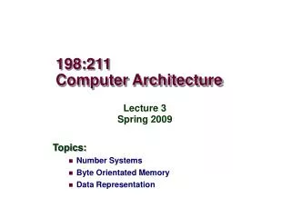
CPU Arithmetic and Login Unit Computer Registers I/O System Bus CPU Internal CPU Interconnection Memory Control Unit CPU Structure • The CPU is the most interesting and most complex component . • Major components: • Control Unit: Controls the operation of the CPU (& therefore the entire computer. • Arithmetic and Logic Unit (ALU): Performs data processing functions. • Registers: Provides storage internal to the CPU. • CPU Interconnection: Provides communication between control unit, ALU, and registers.
A Brief History of Computers http://clio.unice.fr/~monicarm/archi/when.htm The Abacus3000BC Charles Babbage’s Difference Engine 1823
A Brief History of Computers • ENIAC (Electronic Numerical Integrator and Computer) • Designed by Mauchly and Eckert • University of Pennsylvania • First general-purpose electronic digital computer • Response to WW2 need to calculate trajectory tables for weapons. • Built 1943-1946 – too late for war effort. • ENIAC DetailsDecimal (not binary) • 20 accumulators of 10 digits • Programmed manually by switches • 18,000 vacuum tubes • 30 tons • 15,000 square feet • 140 kW power consumption • 5,000 additions per second Vacuum Tube
Von Neumann Machine • Stored Program Concept • Main memory storing programs and data • ALU operating on binary data • Control unit interpreting instructions from memory and executing • Input and output equipment operated by control unit • Princeton Institute for Advanced Studies (IAS). • Completed 1952 Dr. Von Neuman with the IAS computer
Memory of the IAS • 1000 storage locations called words. • Each word 40 bits. • A word may contain: • A numbers stored as 40 binary digits (bits). • An instruction-pair. Each instruction: • An opcode (8 bits) • An address (12 bits) – designating one of the 1000 words in memory.
IAS Instruction set (continued) Example of an Instruction-pair. LoadM(100), AddM(101)0000000100011111010000000101000111110101
Von Neumann Machine Registers • MBR: Memory Buffer Register- contains the word to be stored in memory or just received from memory. • MAR: Memory Address Register- specifies the address in memory of the word to be stored or retrieved. • IR: Instruction Register - contains the 8-bit opcode currently being executed. • IBR: Instruction Buffer Register- temporary store for RHS instruction from word in memory. • PC: Program Counter - address of next instruction-pair to fetch from memory. • AC: Accumulator & MQ: Multiplier quotient - holds operands and results of ALU ops. AC MQ MBR IBR PC IR MAR
Start Is next instructionin IBR? Yes No MAR PC No memoryaccessrequired MBRM(MAR) FETCH CYCLE Leftinstructionrequired? No Yes IR IBR(0:7)MAR IBR(8:19) IR MBR(20:27)MAR MBR(28:39) IBR MBR(20:39)IR MBR(0:7)MAR MBR(8:19) PC PC + 1 Execution Cycle EXECUTION CYCLE
Is next instructionin IBR? Yes No MAR PC No memoryaccessrequired MBRM(MAR) Leftinstructionrequired? FETCH CYCLE No Yes IR IBR(0:7)MAR IBR(8:19) IR MBR(20:27)MAR MBR(28:39) IBR MBR(20:39)IR MBR(0:7)MAR MBR(8:19) PC PC + 1 • MEMORY • 1. LOAD M(X) 500, ADD M(X) 501 • 2. STOR M(X) 500, (Other Ins) • ..... • 3 • 4 PC 2 1 MAR 2 501 500 500 1 MBR STOR M(X) 500, (Other Ins) LOAD M(X) 500, ADD M(X) 501 IR LOAD M(X) ADD M(X) STOR M(X) IBR ADD M(X) 501 (Other Ins) AC 3 7
A Couple of Problems to Solve • Find the average of three numbers. • Let A = A(1), A(2),...,A(10) be a vector containing 10 numbers.Write a a program using the IAS instruction set to sum the numbers in the vector.
2nd Generation: Transistor Based Computers • Transistors replaced vacuum tubes • Smaller • Cheaper • Less heat dissipation • Solid State device • Made from Silicon (Sand) • Invented 1947 at Bell Labs • William Shockley et al. • Commercial Transistor based computers: • NCR & RCA produced small transistor machines • IBM 7000 • DEC – 1957 (PDP-1) First transistor computer – Manchester University 1953.
3rd Generation: Integrated Circuits • A single, self-contained transistor is called a discrete component. • Transistor based computers – discrete components manufactured separately, packaged in their own containers, and soldered or wired together onto circuit boards. • Early 2nd generation computers contained about 10,000 transistors – but grew to hundreds of thousands!!!! (Manufacturing nightmare). • Integrated circuits revolutionized electronics. Silicon Chip – Collection of tiny transistors
Basic Elements of a Digital Computer • Gates • Memory cells • 4 Basic Functions • Data storage (Memory Cells) • Data processing (Gates) • Data movement (Paths between components) • Control (Paths between components)
Manufacturing Integrated Circuits • Thin wafer of silicon divided into a matrix of small areas. • Identical circuit pattern is fabricated onto each area. • Wafer is broken up into chips. • Each chip contains many gates and/or memory cells + input/output attachment points. • Each chip is packaged. • Several packages are then interconnected on a circuit board. A Wafer divided into dies.Photo taken from http://www.computer-tutorial.de/process/cpu3.html
Generations of Computers • Vacuum tube - 1946-1957 (One bit Size of a hand) • Transistor - 1958-1964 (One bit Size of a fingernail) • Small scale integration - 1965 onUp to 100 devices on a chip • Medium scale integration - to 1971100-3,000 devices on a chip • Large scale integration - 1971-19773,000 - 100,000 devices on a chip • Very large scale integration - 1978 to date100,000 - 100,000,000 devices on a chip • Ultra large scale integrationOver 100,000,000 devices on a chip Thousands of bits on the size of a hand Millions of bits on the size of a fingernail.
Moore’s Law • Moore observed that the number of transistors per chip DOUBLED each year. • Predicted the pace would continue. • Since 1975 double every 18 months. • The cost of a chip almostunchanged. cost of logicand memory decreased. • Logic and memoryelements moved closertogether. SPEED. • Computer becomes smaller. more uses. • Reduction in powerand cooling requirements. • Interconnections on ICmore reliable than soldered connections. Fewer interchip connections.
Present Day Computers • Most contemporary computer designs based on Von Neumann architecture. • Three key concepts: • Data and instructions stored in a single read-write memory. (Main Memory) • Contents of memory are addressable by location regardless of the type of data stored there. • Execution occurs in a sequential fashion from one instruction to another (unless modified by a branch etc)
Designing for Performance • Cost continues to drop dramatically. • Performance and capacity continues to rise. • Moore’s law continues to bear out – a new generation of chips unleashed every three years (with 4X as many transistors). • Raw speed useless unless the processor can be fed sufficient work to keep it busy: • Branch prediction • Data flow analysis • Speculative execution
Performance Balance • Processor power raced ahead • Mismatch with other critical components such as main memory. Speed with which data can be accessed and therefore transferred to the processor has lagged.
Trends in DRAM use For a fixed size memory, the number of DRAMs needed is going down – because DRAM density is increasing. At the same time, the amount of memory needed is increasing.
Example borrowed from: http://www.cs.berkeley.edu/~pattrsn/252S98/#projects
Amdahl’s Law • The performance to be gained from using some faster mode of execution is limited by the fraction of the time the faster mode can be used. • Speedup = Execution time for entire task without using the enhancement • Execution time for the entire task using the enhancement when possible. • We need to know two critical factors: • The fraction of the computation time in the original machine that can be converted to take advantage of the enhancement.Fractionenhanced = Enhanced time • Non enhanced time • If a program takes 60 seconds to execute and 20 seconds can be enhanced – then fractionenhanced = 20/60. • The improvement gained by the enhanced execution mode. How much faster will the task run if the enhanced mode were used for the entire program?Speedupenhanced = Time of original mode • Time of enhanced mode
100 seconds 60 seconds not enhanced 40 seconds can be enhanced 60 seconds not enhanced 20 secs after enhance Amdahl’s Law • The execution time using the original machine with the enhanced mode will be the time spent using the unenhanced portion of the machine plus the time spent using the enhancement. Original Execution time Execution time following enhancement • Speedupenhanced = Time of original mode = 100 = 1.25 • Time of enhanced mode 80
Fractionenhanced Speedupenhanced 100 seconds 60 seconds not enhanced 40 seconds can be enhanced 60 seconds not enhanced 20 secs after enhance Amdahl’s Law • Execution timenew = Execution timeold * (1 – Fractionenhanced + 0.4 (40/20) • Execution timenew = 100 * (1 – 0.4 + • = (100 * 0.6) + (100 * (0.4 / 2)) • = 60 + 20 • = 80 seconds • Speedupoverall = 100/80 = 1.25
1 • Speedupoverall = = Fractionenhanced Speedupenhanced Execution timeold Execution timenew • (1 – Fractionenhanced + Amdahl’s Law • Example # 1: (Hennessy & Patterson page 30) • Suppose we were considering an enhancement that runs 10 times faster than the original machine, but is only usable 40% of the time. • What is the overall speedup gained by incorporating the enhancement?
1 • Speedupoverall = = Fractionenhanced Speedupenhanced Execution timeold Execution timenew • (1 – Fractionenhanced + • Example # 2: (Hennessy & Patterson page 31) • Implementations of floating-point (FP) square root vary significantly in performance. Suppose FP square root (FPSQR) is responsible for 20% of a critical benchmark on a machine. • One proposal is to add FPSQR hardware that will sped up this operation by a factor of 10. • The other alternative is just to try to make all FP instructins run faster; FP instructions are responsible for a total of 50% of execution time. • The design team believes that they can make all FP instructions run two times faster with the same effort as required for the fast square root. • Compare these two design alternatives.
Chapter 3: Computer Components – Top Level View • PC = Program Counter • IR = Instruction Register • MAR = Memory AddressRegister • MBR = Memory Buffer Register • I/O AR = I/O AddressRegister • I/O BR = I/O Buffer Register
Basic Function • Basic function is executing a set of instructions stored in memory. • The processor fetches instructions from memory one at a time and executes each instruction. • Program execution therefore consists of repeatedly fetching and executing instructions. • The processing of a single instruction is called the instruction cycle. • The instruction cycle consists of the fetch cycle and the execute cycle.
A Hypothetical Machine • Single data register (AC) • Instructions and data are 16 bits long. • Memory organized as 16 bit words. • Instruction format provides: • 4 bits for the opcode24 = 16 different opcodes. • 12 bits for memory address212 = 4096 (4K) words of memory directly addressable.
Instruction Cycle • Some computers have instructions that contain more than one memory address. • Therefore an instruction cycle may have more than one memory fetch.Example: PDP-11 instruction ADD B,A is equivalent to (A = A + B) • Fetch ADD instruction • Read contents of memory location A into the processor. • Read contents of memory location B into the processor. (ie 2 registers needed!) • Add two values (A + B) • Write result to memory location A. • An instruction may also specify and I/O operation.
Instruction CycleStateDiagram • Instruction address calculation (iac): Determine address of next instruction. • Instruction fetch (if): Read instruction from memory into the processor. • Instruction operation decoding (iod): Analyze instruction to determine type of operation and operand(s) to use. • Operand address calculation (oac): If the operation involves referencing an operand in memory or via I/O – determine the address of the operand. • Operand fetch: Fetch operand from memory or read it from I/O. • Data operation (do): Perform the operation in the instruction. • Operand store (os): Write the result to memory or I/O
Administration • Office HoursThursday 3.30 – 5.00pm or by appointment • Contactemail: jhuang@cs.depaul.edu (preferred)voice mail: 312-362-8863 • Course website: http://facweb.cs.depaul.edu/jhuang/csc345/