Perfect Competition in the

1. Perfect Competition in the Short Run

2. Perfect competition Firms in the real world make either one product or make more than one product. They also may be the only one to make a product or other firms may also make the product(s). When you look at one product, if a firm is one of many firms making the product, and there are many consumers of the product, then the market for the product is said to be perfectly competitive. Let’s focus on the market and how a firm in the market operates. NOTE: a firm is a small part of the competitive market. In other words, any one firm does not make a very large part of the output in the market.

3. Supply and demand The model of supply and demand we have already seen is really the model of perfect competition. We will expand on that idea and focus our attention on a typical firm in that environment. NOTE: we say in economics the GOAL OF THE Firm is to MAXIMIZE PROFIT. This means when the firm looks at all its options it goes for the point or place where profits are a maximum.

4. Revenue potential The market demand curve is downward sloping - in the whole market consumers will buy more at lower prices. But, let’s say for any one firm the demand curve for the firm’s output is horizontal. Why? Any one seller is small relative to the market. 1) If the seller tries to charge a price higher than the market price no one will buy from them(because there are enough other places to buy), and 2) The seller will not charge a lower price because they can sell all they want at the going price. The reason for this is because they are a small part of the market and already sell all they want at the going price.

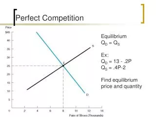
5. Revenue potential P P d P1 D Q Q market Firm The ideas on the previous screen have the graphical interpretation shown here. The demand curve for the firm’s output is a horizontal line at the price that occurs in the market(assumed here to be P1).

6. Revenue potential Since the firm in a competitive environment can not influence the market price on its own, the firm is said to be a price taker and this has implications for the revenue the firm can generate from sales of units of output. Note: since the demand for the firm’s output on the previous screen is horizontal it is said the demand is perfectly elastic. This means if the firm charges any other price the quantity change would be extreme.

7. Revenue potential Total Revenue = TR = P times Q. For the firm here, P is a given value. As an example say P = 2. Units TR of output Notice the change in TR as 0 0 output changes is 2. This is 1 2 called the marginal revenue. 2 4 3 6 So the MR = P = firm demand 4 8 for a competitive firm.

8. Revenue potential As another example say P = 5. Units TR of output Notice the change in TR as 0 0 output changes is 5. Thus 1 5 marginal revenue = 5. 2 10 3 15 So the MR = P = firm demand 4 20 for a competitive firm.

9. review cost concepts $/unit MC AC The cost curves look this way in the short run due to diminishing returns. I picked Q = 30 arbitrarily. At this Q the height of the b AVC a Q or units 30 MC curve is the MC of this output and the height of the AVC and AC curves have similar interpretations. AC minus AVC equals AFC. Area a = TVC, a + b = TC

10. production rule The profit maximizing firm will choose to produce the quantity of output where MR = MC(Q2 in graph). If the firm stops short of the rule, like at Q1, then the firm $/unit MC P = MR Q or units Q1 Q2 Q3 sacrifices units of output where MR > MC. In other words, some units after Q1 add more to revenue than to cost. A profit max. firm wouldn’t pass up this opportunity.

11. production rule If the firm produces beyond Q2, MC > MR and the firm would thus add more to cost than to revenue on these units. A profit maximizing firm would not want to do this. Since the firm goes to where MR = MC and since MR = P for a competitive firm, we see the competitive firm when it maximizes profit has P = MC. (This is a big idea – bells and whistles are sounding, lights are flashing!!!) Since the firm can not do anything about the price, it just adds to production until its MC of production reaches the market price.

12. operating rule The operating rule is a qualification to the production rule. If operating is worth it at all, follow the production rule. Otherwise, shutdown. Now, in the short run there are fixed costs and variable costs. The fixed costs must be paid whether production is 0 or 1,000,000 or whatever. Variable costs must be paid only if variable inputs are employed. It is useful to think of hiring variable inputs only if they generate enough revenue to pay for themselves plus pay for some of the fixed costs. On the next few screens I want to present cases to see what the firm should do: operate or shutdown.

13. operating rule case 1 $/unit MC AC The firm is a price taker - say it takes P P MR a b AVC This firm should operate where MR = MC and make a positive profit c Q or units Q1 If firm operates if it shuts down TR = a + b + c TR = 0 TC = b + c TC = TFC = b profit = a profit = -b.

14. operating rule case 2 $/unit MC AC The firm is a price taker - say it takes P d MR P This firm should operate where MR = MC and have a loss, but not as big as if it shutdown. e AVC f Q or units Q1 If firm operates if it shuts down TR = e + f TR = 0 TC = d + e + f TC = TFC = d + e profit = -d profit = -d -e.

15. operating rule case 3 $/unit MC AC The firm is a price taker - say it takes P g This firm should shutdown. Where MR = MC there is too big a loss, more than if the firm would shutdown. AVC h MR P i Q or units Q1 If firm operates if it shuts down TR = i TR = 0 TC = g + h +i TC = TFC = g profit = -g -h profit = -g.

16. operating rule From these examples we can see that if the price is everywhere below the AVC curve the firm should shutdown. The firm will still have fixed costs to pay, but in this case revenue not only does not pay all fixed costs, it covers only some of variable costs. It is better to shutdown in this case. Shutdown rules: At the Q where P = MC shutdown (sometimes called do not operate) if 1) TR < TVC, or P times Q < TVC, or 2) P < AVC (remember AVC = TVC/Q).

17. firm and market short run supply curve A supply curve is a curve that shows combinations of price and quantity the firm is willing to supply. In other words, we see the quantity the firm is willing to make available for sale at each price. The short run supply curve is the segment of the MC curve that is above the AVC curve. We see this on the next screen IN a competitive market the supply curve is just the summation of the supply curves of the firms. As such, the market supply is really just the addition of marginal cost curves of the individual firms.

18. firm short run supply curve $/unit MC AC P AVC Q or units If the price the firm accepts is above the AVC, then the MC curve acts as the line that shows the price, quantity relations we previously mentioned. The MC curve above the AVC is the supply curve of the firm.