Perfect Competition in the

1. Perfect Competition in the LONG RUN

2. Useful diagram P D1 S1 ATC1 MC1 P1 P=MR1 Q q Q1 q1 Market Firm

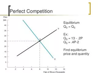
3. Produce the q where MR = MC and see what type of profit exists by looking at (P - ATC) times Q or TR-TC at the q mentioned. Profit = TR - TC PQ = TRATC times Q = (TC/Q) times Q = TC (P-ATC) times Q = PQ - (ATC times Q) = TR - TC

4. Notes about diagram Market In the market the price is determined by the interaction of supply and demand. When you think about the supply curve, there are a certain number of firms involved. You can think of this as being the short run where the amount of capital is fixed for each seller. In the short run, then, no new firms can enter the market either since they can’t get more capital.

5. Notes about diagram Firm The firm will produce where MR = MC and have profit = (P - ATC)Q = 0. SOOOOOOOOOOOO, In the useful diagram, There are only a certain number of firms in the market – say there are x number of firms, where x is a number! The firm we see on the right has profit = 0 because with P = ATC, (P – ATC)Q = 0Q = 0.

6. increase demand On the next screen you will see demand increase in the market. Imagine consumers demand more. Then, 1) The price in the market will increase to P2, 2) The MR(price) for the firm will rise to MR2, 3) The output of the firm will expand to q2, 4) The firm will have profit given by the shaded rectangle.

7. increase demand P D2 D1 S1 ATC1 MC1 P2 P2 = MR2 P1 P1=MR1 Q q Q1 q1 q2 Market Firm

8. demand increase In the short run when the demand increases, existing firms find it worthwhile to produce more, but they can not expand the production facility, by definition, and other firms can not enter the industry. The profit that exists in the short run are enjoyed by the firms in the industry. But in the long run other firms can enter the industry, as well as have existing firms expand their production facility. In the long run we want to note 1) what impact profit has on firms and 2) what happens to input prices.

9. profit impact In the long run positive economic profit attracts firms to the industry. Firms will enter the industry until profit is driven to zero. The presence of economic losses(negative profits) forces some firms to leave the market. Firms will exit until the profit is zero. This is an IMPORTANT SLIDE! Why? Because I spent time typing it – no, er, I mean, cough cough – the logic is that in a competitive environment where it is relatively easy for firms to enter or exit in the long term, profit attracts firms in their attempt to capture some of these profits. Losses in the long term have some firms get out to cut their losses.

10. input prices By definition in economics, resources are scarce. In the context of increasing demand for output we want to think about what might happen to the price of inputs. We consider three cases. 1) Inputs are relatively abundant and thus there is no increase in input prices as the demand for inputs increases. This is called a constant cost industry. 2) Inputs are in relative short supply and thus there is an increase in input prices as the demand for inputs increases. This is called an increasing cost industry. 3) Inputs can be used in new ways and thus there is a decrease in input prices. This is called a decreasing cost industry.

11. ideas to come Now, if a firm has positive economic profit we will see 1) firms enter the market and thus market price falls, and 2) the firms cost curves may shift if input prices change. This will have an impact on how much the supply curve shifts.

12. no change in input prices P D2 D1 S1 ATC1 MC1 S2 P2 P2 = MR2 P1 P1=MR1 Q q Q1 Q2 q1 q2 Market Firm

13. no change in input prices Since there is no change in input prices in this example profit will again be zero when the supply shifts out as far as the new demand to return the price to P1. Supply S1 had a certain amount of firms involved and then some more firms entered(when profit was positive) to give us a certain amount of firms involved with S2. So there really is a separate supply curve for each specific number of firms in the industry. So in the long run we have variation in the number of firms in the industry, depending on the level of demand.

14. Long run supply curve The long run supply curve in the market shows us the price and quantity combinations where 1) the number of firms adjusts, and 2) profit is zero. On the slide two screens ago we see the same price, P1, but two levels of output, Q1 and Q2. Since input prices didn’t change, P1 will always be the price that results in zero profit. On the following screen you will see the long run supply curve in the market in this constant cost case.

15. no change in input prices P D2 D1 S1 ATC1 MC1 S2 P2 P2 = MR2 P1 P1=MR1 Q q Q1 Q2 q1 q2 Market long run supply Firm

16. input prices rise P D2 MC2 ATC2 D1 S1 S2 ATC1 MC1 P2 P2 = MR2 P3 P1 P1=MR1 Q q Q1 q1 q2 Market Firm

17. input prices increase Since input prices increase in this example profit will again be zero when the supply shifts out, but not as far as the demand. Since the cost curves shift up the price to have zero profit will be higher than P1. Here you see the price is P3. Thus supply must shift out to have price P3.

18. input prices rise P D2 MC2 ATC2 D1 S1 S2 ATC1 MC1 P2 P2 = MR2 P3 P1 P1=MR1 Q q Q1 q1 q2 long run supply Market Firm

19. input prices fall P D2 D1 S1 ATC1 MC1 P2 P2 = MR2 S2 P1 P1=MR1 ATC2 MC2 Q q Q1 q1 q2 Market Firm

20. input prices fall Since input prices decrease in this example profit will again be zero when the supply shifts out, but farther than the demand. Since the cost curves shift down the price to have zero profit will be lower than P1. Here you see the price is P4. Thus supply must shift out to have price P4.

21. input prices fall P D2 D1 S1 ATC1 MC1 P2 P2 = MR2 S2 P1 P1=MR1 ATC2 MC2 Q q Q1 q1 q2 Market long run Firm supply

22. long run supply We see the market supply curve is flatter in the long run that in the short run because in the long run firms can enter or exit the industry in response to positive or negative profit.

23. Back to the Useful diagram P D1 S1 ATC1 MC1 P1 P=MR1 Q q Q1 q1 Market Firm

24. Efficiency Efficiency in economics has to do with producing whatever we produce at lowest cost (call productive efficiency), but also producing those things that society most wants (called allocative efficiency). Let’s check out these ideas, shall we? Notice the firm in the useful diagram produces q1 where MR = MC. Since P = MR this is also the q where P = MC. Since profit is driven to zero we know P = ATC. So at q1 we have P = MR = MC = ATC. One last detail. When ATC = MC we know ATC is at a minimum. So in the LR in competition P = MR = MC = min ATC.

25. A joke, then let’s get serious There are 3 kinds of people in the world, those who can count and those who can’t. So in the LR in competition for the firm P = MR = MC = min ATC. This is a triple equal sign. Productive efficiency requires goods be produced in the least costly way. Since P = min ATC goods get produced as cheaply as possible. The min ATC is as low as you can get! Competition in the LR ensures productive efficiency!

26. Allocative efficiency P = MC You might recall the idea of opportunity cost. This is the value of what is given up when a course of action is taken. Notice up to the output level Q1 in the market that the demand curve is above the price and the price is what the consumer pays. Resources go into making the good or service here and the height of the demand curve is essentially indicating how the resources are valued here and not elsewhere. The supply curve and associated MC curve are an indication of how the resources would be valued elsewhere. On all the units up to Q1 the resources used to make them are more value here than elsewhere!!!!

27. Consumer and Producer Surplus Another way to see efficiency is that consumer and producer surplus are maximized in the competitive market outcome!