Download
1 / 13
130 likes | 405 Vues
The table below gives the pretest and posttest scores on the MLA listening test in Spanish for 20 high school Spanish teachers who attended an intensive summer course in Spanish. Teacher Pretest Posttest Teacher Pretest Posttest 1 30 29 11 30 32

E N D
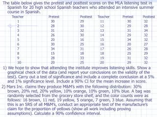
The table below gives the pretest and posttest scores on the MLA listening test in Spanish for 20 high school Spanish teachers who attended an intensive summer course in Spanish. Teacher Pretest Posttest Teacher Pretest Posttest 1 30 29 11 30 32 2 28 30 12 29 28 3 31 32 13 31 34 4 26 30 14 29 32 5 20 16 15 34 32 6 30 25 16 20 27 7 34 31 17 26 28 8 15 18 18 25 29 9 28 33 19 31 32 10 20 25 20 29 32 1) We hope to show that attending the institute improves listening skills. Show a graphical check of the data (and report your conclusions on the validity of the test). Carry out a test of significance and include a complete conclusion at a 5% and 1% significance level. Include a 90% CI for the mean increase in score. 2) Mars Inc. claims they produce M&M’s with the following distribution: 30% brown, 20% red, 20% yellow, 10% orange, 10% green, 10% blue. A bag was randomly selected from the grocery store shelf, and the color counts were as follows: 16 brown, 11 red, 19 yellow, 5 orange, 7 green, 3 blue. Assuming that this is an SRS of all M&M’s, conduct an appropriate test of the manufacture’s claim for the proportion of yellows (show all work including proving assumptions). Calculate a 90% confidence interval.
14.1 Goodness of Fit • Suppose you open a 1.69 ounce bag of plain M&M chocolate candies and discover that out of 56, there is only one blue M&M. • Knowing that 10% of all M&M’s are blue and that out of your sample only 1/56 = .018 are blue, we might want to use the z-test to test the hypothesis that Ho: p = .10 Ha: p < .10 where p is the proportion of blues. We could then perform additional tests of significance for each of the remaining colors.
Chi-Squared Test (for goodness of fit) • A single test that can be applied to see if the observed sample distribution is different from the hypothesized population distribution. • Also used to test if all proportions in a set of data are equal, or at least two proportions in a set of data is not equal.
Family of distributions that.. • Take only positive values (starts at 0 on horizontal axis, increases to a peak, and then approaches the horizontal axis asymptotically from above) • Skewed to the right (as df increases, curve becomes more symmetrical and looks more like a normal curve) • Total Area under curve = 1 • One parameter: df.
In recent years, the expression “The graying of America” has been used to refer to the belief that w/better medicine and healthier lifestyles, people are living longer (and consequently, a larger % of the pop. is of retirement age). Investigate whether this perception is accurate. Example
Chi-Squared Test Statistic • In order to determine whether the distribution has changed since 1980, we need a way to measure how well the observed counts (O) from 2006 fit the expected counts (E) under Ho.
Observed Counts (given): Sample results for 500 randomly selected individuals in 2006
Using the TI-83 • Clear lists L1, L2, L3 • Enter observed counts in L1 (177, 158, 101, 64) • Enter expected counts in L2 (207, 138.4, 98.2, 56.4) • Program L3 = ((L1-L2)^2)/L2 • Sum L3 (2nd/LIST/MATH/5:sum) • 2nd Vars (Distributions Menu), 7: Chi-Squared cdf(8.277, 1E99 (large#), df=3) • Resulting pvalue indicates 8.277 is unlikely result if Ho is true; strong evidence against Ho.
Conclusion • The probability of observing a result as extreme as the one we got (by chance) is between 2 and 5%. • Therefore, the population distribution in 2006 is significantly different from the 1980 distribution.
More TI-83: Chi-Square Density Curves • Window: 0, 14, 1, -.05, .3, .1, 1 • Y1: 2nd Dist (chi-squared pdf X,1) • Y2: 2nd Dist (chi-squared pdf X,4) • Y3: 2nd Dist (chi-squared pdf X, 8) • Graph individually, then together
The Advanced Placement (AP) Statistics examination was first administered in May 1997. Students’ papers are graded on a scale of 1 to 5, with 5 being the highest score. Over 7600 students took the exam in the first year, and the distribution of scores was as follows (not including exams that were scored late). Score 5 4 3 2 1 Percent 15.3 22.0 24.8 19.8 18.1 A distance learning class that took AP Statistics via satellite television had the following distribution of grades: Score 5 4 3 2 1 Frequency 7 13 7 6 2 1) Calculate marginal percents and make a bar graph of the population scores and the sample scores on the same grid, so that the two distributions can be compared visually. 2) Carry out an appropriate test to determine if the distribution of scores for students enrolled in the distance-learning program is significantly different from the distribution of scores for all students who took the inaugural exam.