Download

1 / 16
170 likes | 366 Vues
13.1 Goodness of Fit Test. AP Statistics. Chi-Square Distributions. The chi-square distributions are a family of distributions that take on only positive values and are skewed to the right . A specific chi-square distribution is determined by its degrees of freedom. Properties :.

E N D
13.1Goodness of Fit Test AP Statistics
Chi-Square Distributions The chi-square distributions are a family of distributions that take on only positive valuesand are skewed to the right. A specific chi-square distribution is determined by its degrees of freedom.
Properties: • The total area under a chi-square curve is equal to 1. • Each chi-square curve (except when df = 1) begins at 0 on the horizontal axis, increases to a peak, and then approaches the horizontal axis asymptotically from above. • Each chi-square curve is skewed to the right. As the number of degrees of freedom increase, the curve becomes more and more symmetrical and looks more like a normal curve (see Figure 13.2 page 732 ).
According to the m&m/Mars company, in 1995 “…the new mix of colors of m&m’s plain chocoloate candies will contain 30 percent browns, 20 percent yellows and reds, and 10 percent each of oranges, greens, and blues.” However, the mix of colors has been known to change every few years. Your task today is to determine whether or not the current mix of colors matches that of 1995. We want to see if there is sufficient evidence to reject the company’s 1995 claim. To do this, we’ll be introduced to a new type of test—the Chi-square Goodness of Fit Test.
A Goodness of Fit Test is used to determine whether a population has a certain hypothesized distribution. The null hypothesis is that the population proportions are equal to the hypothesized proportions. The alternative is that at least one of the proportions differfrom the hypothesized proportions. If all expected counts are at least 1 and 80% of them are greater than 5, then has an approximately Chi-Square Distribution with df = (k – 1).
Open a bag of milk chocolate m&m’s and carefully count how many of each color are in the sample. Record the observed data in the “observed” row of the table below. • Using the statement from the m&m/Mars company, determine how many of each color you expected to see. Note, you’ll have to figure this out using the total number of m&m’s in your sample bag. Enter these counts in the “expected” row below.
If your bag reflects the distribution advertised in 1995, there should be little difference between the observed and expected counts. To quantify the difference we’ll calculate a total which we’ll call “Chi-Square” or X2. • For each color, perform this calculation: Enter each value in the last row of the table. Add up all of these “component” values to find X2. • If this total value is small, we have little evidence to suggest a difference in distributions. However, the larger X2 gets, the more evidence we have to suggest the company’s claim may no longer be applicable to bags of milk chocolate m&m’s.
To determine the likelihood of observing a difference between observed and expected as extreme as the one we observed, we must look up the p-value on a Chi-Square table. Chi-square distributions are skewed right and specified by degrees of freedom. In a Goodness of Fit test, the degrees of freedom equal one less than the number of categories.
Find the p-value for our test by looking up X2 for 5 degrees of freedom. Sketch the curve and observed X2 below. Interpret the result in the context of the problem. X2cdf(X2, 1E99, df) Since p is large (> α), there is not significant evidence to reject the 1995 claim.
Steps: • Identify the population of interest and the parameter(s) that you want to draw conclusions about. State hypotheses in words and symbols. • Choose the appropriate inference procedure and verify the conditions for using it. Chi-Square Conditions: • All individual expected counts are at least 1 • No more than 20% of the expected counts are less than 5 • Carry out the inference procedure (calculate the T.S., df, and p-value). • Interpret your results in the context of the problem.
Example 1: (13.13 p. 744) A “wheel of fortune” at a carnival is divided into four equal parts: Part I: Win a doll Part II: Win a candy bar Part III: Win a free ride Part IV: Win nothing You suspect that the wheel is unbalanced (i.e., not all parts of the wheel are equally likely to be landed upon when the wheel is spun). The results of 500 spins of the wheel are as follows: Part: I II III IV Frequency: 95 105 135 165 Perform a goodness of fit test. Is there evidence that the wheel is not in balance?
Since the wheel is divided into four equal parts, if it is in balance, then the four outcomes should occur with approximately equal frequency. Here are the observed and expected values: Part: I II III IV Observed: 95 105 135 165 Expected: 125 125 125 125 Ho: The wheel is balanced (the four outcomes are uniformly distributed) Ha: The wheel is not balanced We will use a chi-square goodness of fit test to measure the strength of the evidence against the hypothesis that the wheel is balanced. Since all expected counts are greater than 5, we can proceed with the test. df = 3 X2cdf(24, 1E99, 3) p < α Reject Ho We have significant evidence to conclude that the wheel is not balanced. Since “Part IV: Win nothing” shows the greatest deviation from the expected result, there may be reason to suspect that the carnival game operator may have tampered with the wheel to make it harder to win.
Example 2:A statistics student suspected that his 1982 penny was not a fair coin, so he held it upright on a table top with a finger of one hand and spun the penny repeatedly by flicking it with the index finger of his other hand. In 200 spins of the coin, it landed with tails side up 122 times. (a) Perform a goodness of fit test to see if there is sufficient evidence to conclude that spinning the coin does not produce an equal proportion of heads and tails. Ho : The distribution of heads and tails from spinning a 1982 penny shows equally likely outcomes. Ha : Heads and tails are not equally likely. We will use a chi-square goodness of fit test to measure the strength of the evidence against the hypothesis that the penny is a fair coin. Since all expected counts are greater than 5, we can proceed with the test. df = 1 p < α Reject Ho We have significant evidence to conclude that spinning a 1982 penny does not produce equally likely results.
(b) Use a one-proportion inference procedure to determine whether spinning the coin is equally likely to result in heads or tails. p = probability of getting tails when the coin is spun Ho : p = 0.5 Ha : p ≠ 0.5 Assume SRS. Assume population > 10(200) np = n(1-p) = 100 > 10 1-prop-z-test p < α Reject Ho. There is significant evidence to conclude that heads and tails are clearly not equally likely (α = 0.05)
(c) Compare your results for parts (a) and (b). The p-values are identical. Same conclusion.