Download
1 / 18
190 likes | 390 Vues
Goodness of Fit. What is Chi Squared How to use it with more than 2 proportions. Introduction; Test of goodness of fit. What is Goodness of Fit (GoF) ? We have a population. We claim that the population has a specific distribution . We check if we could reject that claim.

E N D
Goodness of Fit • What is Chi Squared • How to use it with more than 2 proportions
Introduction; Test of goodness of fit What is Goodness of Fit (GoF) ? We have a population. We claim that the population has a specific distribution. We check if we could reject that claim. Select a sample and Collect data. Compare sample results with those that are expected when the null hypothesis is true. The conclusion of hypothesis test is based on how close the sample results are to the expected results.
Example : multinomial population Over the past year market shares have stabilized at Company Market share % A 30 B 50 C 20 This is a multinomial distribution. Recently, company C has developed a new product. We want to know whether the new product has changed the market share or not. We should conduct a goodness of fit test.
Example : multinomial population • Multinomial Distribution Goodness of Fit Test Let pA = market share for company A pB = market share for company B pC = market share for company C Hypotheses H0:pA = .3, pB = .5, pC = .2 Ha: The market shares are notpA = .3, pB = .5, pC = .2
Sampling If the sample results lead to rejection of H0, then we have evidence that that the introduction of the new product has changed the market shares. We have randomly asked 200 customers to specify whether they buy from company A, B, or C. The result is shown below Company Observed frequency (fi) A 48 B 98 C 54 Now we perform a goodness of fit test to will determine whether the sample results is consistent with the null hypothesis or not.
Expected results We should compare observed frequencies with expected frequencies. Given a sample of size 200, and expectations of pA = .3, pB = .5, pA = .2, the expected frequencies are Company Expected frequency (ei) A .3(200) = 60 B .5(200) = 100 C .2(200) = 40 The goodness of fit test concentrates on the difference between observed and expected frequencies. Large differences mean that the null hypothesis in not true. In other words, introduction of the new product by company C has changed the market shares.
Test statistic for goodness of fit We should compare observed frequencies with expected frequencies. fi : observed frequency for category i ei : expected frequency for category i k : the number of classes or categories. The test statistic x2 has a chi-square distribution with k-1 degrees of freedom, provided that the expected frequencies are 5 or more for all categories.
Do Not Reject H0 Reject H0 2 Example; Rejection rule Conclusion We reject the assumption of there is no home style preference, at the .05 level of significance.
Do Not Reject H0 Reject H0 2 Chi-square test statistic calculations The value of the test statistic is 7.34 x2 = 7.34
Chi-square test; rejecting the null hypothesis • We test the null hypothesis at the = .05 level of significance. • Since we reject the null hypothesis for large differences, therefore the rejection area of = .05 is in the upper tail of chi-square distribution • Chi-square distribution table is given in Appendix B table 3. Given the level of significance of = .05, and degree of freedom of k-1=3-1=2, we will find X2.05 = 5.99. • What is the meaning of this 5.99. • It says with a probability of .95 any chi-square variable of this type • has a value less than 5.99.
Do Not Reject H0 Reject H0 2 Chi-square test; rejecting the null hypothesis • Now if the value of our variable is greater than 5.99, there is .05 • probability that it is still from the same distribution. However, there is .95 probability that it is from some other distribution. Therefore with a .05 level of significance we reject it. • Our X2 value was 7.34. • 7.34 > 5.99 ==> null hypothesis is rejected. • New product of company C has changed the market share
P-value Instead of calculating x2,we may calculate p-value. p-value is the probability related to the test statistic. In GoF test, P-value is the probability of having a chi-square variable greater than the test statistic x2. In our example, text statistic is X2 = 7.34. Now we go to chi-square table to see what is the probability related to this X2 value.Note that d.f. is 3-1 = 2. P-value of X2 = 7.34 and 2 d.f. is some ting close to .025.
P-value Then we can compare p-value with, > p-value ===> H0is rejected. If null hypothesis is true, P-value is the probability of obtaining a sample result that is at least as unlikely as what is observed. P-value is often referred to as observed level of significance. = .05 p-value = .025 .05 > .025 ===> H0is rejected.
Multinomialpopulation; Summary 1. Set up the null and alternative hypotheses. 2. Select a random sample and record the observed frequency, fi , for each of the k categories. 3. Assuming H0 is true, compute the expected frequency, ei , in each category by multiplying the category probability by the sample size. 4. Compute the value of the test statistic. 5. Reject H0 if (where is the significance level and there are k - 1 degrees of freedom).
Example; Finger Lakes Homes Finger Lakes Homes manufactures four models of prefabricated homes, a two-story colonial, a ranch, a split-level, and an A-frame. To help in production planning, management would like to determine if previous customer purchases indicate that there is a preference in the style selected. The number of homes sold of each model for 100 sales over the past two years is shown below. Model Colonial Ranch Split-Level A-Frame # Sold 30 20 35 15
Example; Finger Lakes Homes • Multinomial Distribution Goodness of Fit Test Let pC = population proportion that purchase a colonial pR = population proportion that purchase a ranch pS = population proportion that purchase a split-level pA = population proportion that purchase an A-frame Hypotheses H0:pC = pR = pS = pA = .25 Ha:The population proportions are not pC = .25, pR = .25, pS = .25, and pA = .25
Example; Finger Lakes Homes Expected Frequencies e1 = .25(100) = 25 e2 = .25(100) = 25 e3 = .25(100) = 25 e4 = .25(100) = 25 Test Statistic = 1 + 1 + 4 + 4 = 10
Do Not Reject H0 Reject H0 2 7.81 Example; Rejection rule With = .05 and k - 1 = 4 - 1 = 3 degrees of freedom Conclusion We reject the assumption of there is no home style preference, at the .05 level of significance.