Notices
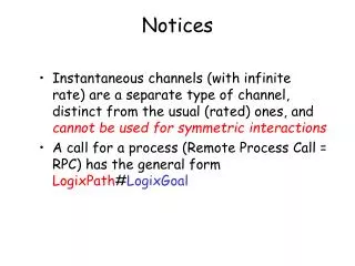
Notices. Instantaneous channels (with infinite rate) are a separate type of channel, distinct from the usual (rated) ones, and cannot be used for symmetric interactions A call for a process (Remote Process Call = RPC) has the general form LogixPath # LogixGoal. Notices.

Notices
E N D
Presentation Transcript
Notices • Instantaneous channels (with infinite rate) are a separate type of channel, distinct from the usual (rated) ones, and cannot be used for symmetric interactions • A call for a process (Remote Process Call = RPC) has the general form LogixPath#LogixGoal
Notices • LogixPath may be the name of a module (e.g. nacl_1) or a transformation of a UNIX path: dir1/dir2/…/dirn/module.cp dir1#dir2#…#dirn#module • LOGIX treats an alphanumeric name which begins with a lower case letter as a string, hence it does not require quotes • Any other names starting with upper case letter (except for Logix variables) require quotes • LogixGoal may be any process defined within the target module. Since BioPSI processes start with upper case letter they must be quoted
Radicals and Functional Groups • Free radicals are highly reactive, typically univalent, “parts” of molecules • Organic compounds are composed of functional groups • A functional group is the the part of a molecule a having special arrangements of atoms that is largely responsible for the chemical behavior of the parent molecule • We focus on reactions involving almost exclusively organic compounds and functional groups
A Modular Approach to Radicals, Groups and Compounds • For a reaction of the type A+B C • We will • Represent A, B as processes • Upon interaction • A, B processes will be terminated • A new process, C, will be spawned • Example: O + H O2 + H2 + H2O
A Modular Approach to Radicals, Groups and Compounds • For reverse unimolecular reaction C A + B • Before, we had two counterparts (Bound_A and Bound_B) which unbound from each other • Now, we have a single reactant process C • In the pi-calculus we are limited to pair wise interactions
A Modular Approach to Radicals, Groups and Compounds • We will add a Timer process that will offer the complementary communication required by the pi-calculus. • We will use a single instance of this process to ensure a correct rate calculation
Condensation and hydrolysis Amine Carboxyl Amide amine eRN eRC eRN eRC hydrolysis R(eRC) R(eRN) R(eRC) R(eRN) NH2(eRN) COOH(eRC) Amide(eRN,eRC)
RNH2 + RCOOH RNHCOR + H2O -language(psifcp).global(amine(10),hydrolysis(1)). R_Amine+eRN::= NH2(eRN) | R(eRN) .R_Carboxyl+eRC::= R(eRC) | COOH(eRC) .NH2(eRN)::= amine ? {eRC1} , Amide(eRN,eRC1) | H2O .Amide(eRN,eRC)::= hydrolysis ? [] , COOH(eRC) | NH2(eRN) .COOH(eRC)::= amine ! {eRC} , true . R(e)::= e ! [] , self .H2O::= hydrolysis ! [] , true . condensation_peptide_1.cp
Unit 3: Programming and Tracing Polymers, Compartments and other Quantitative Aspects
Chain Reaction and Polymerization • Multi-step reaction mechanisms in which certain steps may be repeated indefinitely. • Typically involve three types of steps • Intiation reaction • Chain propagation reaction(s) • Chain termination reaction • Occur in flames, explosions, atmosphetic and life processes, and are important for the creation of synthetic polymers
Monomers Seeds Y Y A A A A A A A A A Y Initiation Propagation Y A* A Y A A* Y A A A* A A Termination Y A A A* Y Y A A A A A A Y A A A* Polymer Polymerization
Synthetic polymers: Polyethylene • InitiationY + CH2=CH2 Y-CH2-CH2* • Propagation Y-(CH2-CH2)n- CH2-CH2* + CH2=CH2 Y-(CH2-CH2)n+1-CH2-CH2* • Termination Y-(CH2-CH2)n- CH2-CH2* + Y-(CH2-CH2)m- CH2-CH2* Y-(CH2-CH2)m+n+2-Y
Polyethylene - Initiation alkene_Y polyCC polyCC_L polyCC_R Y + CH2=CH2 Y----CH2-CH2* Y+polyCC Ethylene Bound_Y(polyCC) EthylR(polyCC_L)+ polyCC_R
Polyethylene - Propagation pCC_R pCC_L +pCC_R pCC pCC_L pCC_R pCC_L Y-------------(CH2-CH2)------------(CH2-CH2)------------CH2-CH2* + CH2=CH2 Y-(CH2-CH2)2-------- CH2-CH2 -------CH2-CH2* Bound_Y(pCC) EthylP(pCC_L, pCC_R) EthylP(pCC_L , pCC_R) EthylR(pCC_L) +pCC_R Ethylene alkene_R pCC_R pCC_L pCC_R pCC_L +pCC_R EthylP(pCC_L, pCC_R) EthylR(pCC_L) +pCC_R
Polyethylene - Termination pCC_L pCC_L Y-(CH2-CH2)n---- CH2-CH2* + Y-(CH2-CH2)m---- CH2-CH2* Y-(CH2-CH2)n- CH2-CH2 ------CH2-CH2-(CH2-CH2)m- Y EthylR(pCC_L) +pCC_R EthylR(pCC_L) +pCC_R poly_R* pCC_L pCC_R pCC_R pCC_L EthylP_term(pCC_L, pCC_R) EthylP_term(pCC_L, pCC_R) * poly_R is a symmetric channel(either pCC_R or pCC_R could end up as the shared channel)
Polyethylene -language(psifcp).global(dummy, alkene_Y(1), alkene_R(10), poly_R(1)).System(N1,N2)::= CREATE_Y(N1) | CREATE_Ethylene(N2) . CREATE_Y(C)::= {C =< 0} , true ; {C > 0} , {C--} | Y | self .CREATE_Ethylene(C)::= {C =< 0} , true ; {C > 0} , {C--} | Ethylene | self . Polyethylene_1.cp
Polyethylene Y+polyCC::= alkene_Y ! {polyCC} , Y_bound(polyCC) .Y_bound(polyCC)::= dummy ? [] , true . Ethylene::= alkene_Y ? {polyCC_L} , EthylR(polyCC_L) ; alkene_R ? {polyCC_L} , EthylR(polyCC_L) . EthylR(polyCC_L)+polyCC_R::= alkene_R ! {polyCC_R} , EthylP(polyCC_L, polyCC_R) ; poly_R ! {polyCC_R} , EthylP_term(polyCC_L, polyCC_R); poly_R ? {polyCC_R} , EthylP_term(polyCC_L, polyCC_R). EthylP(polyCC_L, polyCC_R)::= dummy ? [] , true . EthylP_term(polyCC_L, polyCC_R)::= dummy ? [] , true . Polyethylene_1.cp
Initiation Y+polyCC| Ethylene alkene_Y ! {polyCC} , Y_bound(polyCC) |alkene_Y ? {polyCC_L} , EthylR(polyCC_L) ; alkene_R ? {polyCC_L} , EthylR(polyCC_L) . alkene_Y Y_bound(polyCC) | EthylR(polyCC)+polyCC_R Polyethylene_1.cp
Propagation EthylR(polyCC)+polyCC_R | Ethylene alkene_R ! {polyCC_R} , EthylP(polyCC, polyCC_R) ; …| alkene_Y ? {polyCC_L} , EthylR(polyCC_L) ; alkene_R ? {polyCC_L} , EthylR(polyCC_L) . alkene_R EthylP(polyCC,polyCC_R)| EthylR(polyCC_R)+polyCC_R Polyethylene_1.cp
Termination EthylR(polyCC_R)+polyCC_R| EthylR(polyCC_R)+polyCC_R alkene_R ! {polyCC_R} , EthylP(polyCC_R, polyCC_R) ;poly_R ! {polyCC_R} , EthylP_term(polyCC_R, polyCC_R); poly_R ? {polyCC_R} , EthylP_term(polyCC_R, polyCC_R) | alkene_R ! {polyCC_R} , EthylP(polyCC_R, polyCC_R) ; poly_R ! {polyCC_R} , EthylP_term(polyCC_R, polyCC_R);poly_R ? {polyCC_R} , EthylP_term(polyCC_R, polyCC_R). poly_R EthylP_term(polyCC_R, polyCC_R)|EthylR(polyCC_R, polyCC_R) Polyethylene_1.cp
Polyethylene (100 Ethylene ; 2 Y seeds) EthylP EthylR Ethylene Polyethylene_1.cp
Polyethylene(200 Ethylene, 4 Y seeds) EthylP EthylR Ethylene
What Else Would We Like to Trace? • What is the length of each molecule? • What is the position of each of the monomers inside the polymer? • How can we follow the process of polymerization?
Nucleic Acids Base* Phosphate 5’ Base P Sugar 5’ Phosphoester bond 3’ 3’ Sugar (pentose = 5 C) Adenine (here)*; Guanine, Thymine, Cytosine, Uracil
Phosphodiester Bonds and Nucleic Acid Polymerization 3’ 5’ Phosphodiester bond
Nucleic Acid Polymerization is Directional • Polymerization proceeds in the 5’3’ direction: • The 5’ phosphateof a free nucleotide binds to the 3’ growing endof an existing chain • In cells this process requires a complex machinery (as we will learn later on) • For now, we will focus on the chain propagation mechanism.
P Phosphodiester Bonds and Nucleic Acid Polymerization 5’ Seed Free nucleotides 3’ 5’ P 5’ P 3’ 3’ 5’ P 5’ P Polymerized nucleotides 3’ 3’ 5’ P 5’ P 3’ 3’ 5’ P Growing end 3’
Nucleic Acid Polymerization -language(psifcp).global(hydroxyl_P(1)).System(N1,N2)::= << CREATE_Nucleotide(N1) | CREATE_Seed_Nucleotide(N2). CREATE_Nucleotide(C)::= {C =< 0} , true ; {C > 0} , {C--} | Nucleotide | self . CREATE_Seed_Nucleotide(C)::= {C =< 0} , true ; {C > 0} , {C--} | Seed_Nucleotide | self >> . phosphodiester_sugar_phosphate_7a.cp
Nucleic Acid Polymerization Seed_Nucleotide::=<< hydroxyl_P ? {pd_ester} , Seed_Bound(pd_ester) . Seed_Bound(pd_ester)::= pd_ester ! [] , Seed_Nucleotide >> . Nucleotide+pde(0.001)::= << hydroxyl_P ! {pde} , Nucleotide_5_Bound(pde) .Nucleotide_5_Bound(pde)::= pde ? [] , Nucleotide ; hydroxyl_P ? {pd_ester} , Nucleotide_5_3_Bound(pde,pd_ester).Nucleotide_3_Bound(pd_ester)::= pd_ester ! [] , Nucleotide .Nucleotide_5_3_Bound(pde,pd_ester)::= pde ? [] , Nucleotide_3_Bound(pd_ester) ; pd_ester ! [] , Nucleotide_5_Bound(pde) >> . phosphodiester_sugar_phosphate_7a.cp
5’ 3’ pde P 5’ P 3’ Initiation Seed_Nucleotide | Nucleotide+pde hydroxyl_P ? {pd_ester} , Seed_Bound(pd_ester) | hydroxyl_P ! {pde} , Nucleotide_5_Bound(pde) hydroxyl_P pde Seed_Bound(pde) | Nucleotide_5_Bound(pde) pde ! [] , Seed_Nucleotide | pde ? [] , Nucleotide ; … phosphodiester_sugar_phosphate_7a.cp
5’ 3’ pde P 5’ P 3’ 5’ P 3’ Elongation pde Nucleotide_5_Bound(pde) | Nucleotide+pde pde ? [] , Nucleotide ;hydroxyl_P ? {pd_ester} , Nucleotide_5_3_Bound(pde,pd_ester) | hydroxyl_P ! {pde} , Nucleotide_5_Bound(pde) pde hydroxyl_P Nucleotide_5_3_Bound(pde, pde) | Nucleotide_5_Bound(pde) pde ? [] , Nucleotide_3_Bound(pde) ;pde ! [] , Nucleotide_5_Bound(pde) | pde ? [] , Nucleotide ;hydroxyl_P ? {pd_ester} , Nucleotide_5_3_Bound(pde,pd_ester) phosphodiester_sugar_phosphate_7a.cp
5’ P P 5’ 5’ P P 3’ 3’ Cleavage 3’ pde Nucleotide_5_3_Bound(pde, pde) | Nucleotide_5_3_Bound(pde,pde) 5’ P 3’ pde pde ? [] , Nucleotide_3_Bound(pde) ;pde ! [] , Nucleotide_5_Bound(pde) |pde ? [] , Nucleotide_3_Bound(pde) ;pde ! [] , Nucleotide_5_Bound(pde) 5’ P 3’ pde pde 5’ 5’ P Nucleotide_5_Bound(pde) |Nucleotide_3_Bound(pde) 3’ 3’ pde pde 5’ P phosphodiester_sugar_phosphate_7a.cp 3’
P 5’ 3’ 5’ P 3’ 5’ P 3’ P 5’ 3’ 5’ P 3’ Phosphodiester bonds and nucleic acid polymerization 1 Bound Seed + 5 “3_Bound” = 6 “5_Bound” = 6 polypeptides phosphodiester_sugar_phosphate_7a.cp
What Else Would We Like to Trace? • What is the length of each molecule? • What is the position of each of the monomers inside the polymer? • How can we follow the process of polymerization? • Which chains are formed by cleavage?
Exercise 4 – Question 1 • Does the nucleic acid program ensure directionality? Explain your answer
Exercise 4 – Question 2 • A similar directional polymer is formed from monomer amino acids by the creation of a peptide bond. Each amino acid has two functional groups: an amine group and a carboxyl group. The two can form an amide (peptide) bond (See previous lesson). The resulting polymer is a polypeptide.
Exercise 4 – Question 2 • Based on the nucleic acid example, write a program for the formation and cleavage of such “polypeptides” • Assume: • The polypeptide is initiated from a Seed • It is created in a directional fashion COOH (in seed or end of existing polymer) NH2(in incoming monomer): The NH2 group in each amino acid is “enabled” before the COOH group • You should distinguish between Seed, free amino acids, COOH-bound, NH2-bound and COOH AND NH2 bound monomers.
Exercise 4 – Question 2 In addition to the standard (code, record, .table, .names, plot) also determine how many individual chains you have at the end of the run
Quantitative Options • Representing each molecule as a separate process can be costly • In some cases we do not wish to represent each molecule as a separate process, but would rather represent only molecular species as distinct processes • In other cases we would like to follow other quantitative aspects. E.g the location of a nucleotide in a polymer.
Quantitative Options • We will use Logix variables as counters to account for the number of molecules we have in each species • We will use this counters as message multipliers to ensure the correct rate calculation • We can also use counters in processes to represent location (in polymer) or other relevant quantitative properties
Variables • Variables are denoted by alphanumeric strings, beginning with an upper case alphabetic character • The string may contain an underscore character (_) or be a single underscore character. • We may use variables as parameters and in messages (we can mix in one tuple channels and variables) • May be used in various arithmetic and logic operations (e.g. summation, comparison) • We’ve all ready seen some examples in the spawning loop (e.g. {R++} or {R>0} )
Variables • We are using Logix variables, which can be assigned a value only once. Hence, every operation (e.g. R++) creates a new variable, which is assigned the new value • The new variable is local to the process in which the operation was performed, and is distinct from all other variables in other processes (that appear to have the same name)
Na + Cl Na+ + Cl- • Each process: One chemical species (4 process in the system at all times) • A counter is maintained in every process. • The counter is initialized according to the starting quantities • Following each communication the reactant process decrements its own counter and alerts the relevant product process to increment its counter • The counter is used as a message multiplier
Na + Cl Na+ + Cl- language(psifcp).global(e1(90),e2(10)).-baserate(infinite). System(N1,N2,N3,N4)+(e3,e4)::= << Na | Cl | Na_plus | Cl_minus . Na::= e1 ! N1 *[] , {N1--} , e3 ! [] , Na ; e3 ? [] , {N1++} , Na . Na_plus::= e2 ? N3 * [] , {N3--} , e3 ! [] , Na_plus ; e3 ? [] , {N3++} , Na_plus . Cl::= e1 ? N2 * [] , {N2--} , e4 ! [] , Cl ; e4 ? [] , {N2++} , Cl . Cl_minus::= e2 ! N4 * [] , {N4--} , e4 ! [] , Cl_minus; e4 ? [] , {N4++} , Cl_minus >> . <channel> ! <multiplier> * <message> <channel> ? <multiplier> * <message> nacl_1b.cp
What Else Would We Like to Trace? • The values of each Process Counter at each time point
Logix Variables • Variable values can be displayed on the screen or written into a file by using e.g. • screen#display(counter = CA) • screen#display(counter = CA,append(filename)) • Use this command as you would use any other call to a process
Logix Variables language(psifcp).global(e1(90),e2(10)).-baserate(infinite). System(N1,N2,N3,N4)+(e3,e4)::= << Na | Cl | Na_plus | Cl_minus . Na::= e1 ! N1 *[] , {N1--} , e3 ! [] , screen#display(counter=N1,append(count_txt)) |Na ; e3 ? [] , {N1++} , Na . Na_plus::= e2 ? N3 * [] , {N3--} , e3 ! [] , Na_plus ; e3 ? [] , {N3++} , Na_plus . Cl::= e1 ? N2 * [] , {N2--} , e4 ! [] , Cl ; e4 ? [] , {N2++} , Cl . Cl_minus::= e2 ! N4 * [] , {N4--} , e4 ! [] , Cl_minus; e4 ? [] , {N4++} , Cl_minus >> .
Logix Variables autumn:~/Course/->122% + count_txt counter = 3 counter = 2 counter = 1 counter = 2 counter = 1 counter = 0 counter = 1 counter = 0 counter = 0 counter = 2 counter = 2 counter = 1 counter = 1 autumn:~/Course/Electron_1/quant->123%
BioPSI Time • The current time can also be similarly accessed and displayed. • A special FCPprocedure now(Now) is available in status.cp, which put the current time in the variable Now. • The value of this variable can be displayed by the usual procedure