Utility Maximization
Utility Maximization. Continued July 5, 2005. Graphical Understanding. Normal Indifference Curves. Downward Slope with bend toward origin. Graphical. Non-normal Indifference Curves. Y & X Perfect Substitutes. Graphical. Non-normal. Only X Yields Utility. X & & are perfect


Utility Maximization
E N D
Presentation Transcript
Utility Maximization Continued July 5, 2005
Graphical Understanding • Normal Indifference Curves Downward Slope with bend toward origin
Graphical • Non-normal Indifference Curves Y & X Perfect Substitutes
Graphical • Non-normal Only X Yields Utility
X & & are perfect complementary goods Graphical • Non-normal
Calculus caution • When dealing with non-normal utility functions the utility maximizing FOC that MRS = Px/Py will not hold • Then you would use other techniques, graphical or numerical, to check for corner solution.
Cobb-Douglas • Saturday Session we know that if U(X,Y) = XaY(1-a) then X* = am/Px • m: income or budget (I) • Px: price of X • a: share of income devoted to X • Similarly for Y
Cobb-Douglas • How is the demand for X related to the price of X? • How is the demand for X related to income? • How is the demand for X related to the price of Y?
CES • Example U(x,y) = (x.5+y.5)2
CES Demand Eg: Y = IPx/Py(1/(Px+Py)) Let’s derive this in class
I=150 I=100 CES Demand | Px=5 • I=100 & I = 150
Px=10 Px=5 CES | I = 100
For CES Demand • If the price of X goes up and the demand for Y goes up, how are X and Y related? • On exam could you show how the demand for Y changes as the price of X changes? • dY/dPx
When a price changes • Aside: when all prices change (including income) we should expect no real change. Homogeneous of degree zero. • When one prices changes there is an income effect and a substitution effect of the price change.
Changes in income • When income increases demand usually increase, this defines a normal good. • ∂X/∂I > 0 • If income increases and demand decreases, this defines an inferior good.
Normal goods As income increase (decreases) the demand for X increase (decreases)
Inferior good As income increases the demand for X decreases – so X is called an inferior good
A change in Px Here the price of X changes…the budget line rotates about the vertical intercept, m/Py.
The change in Px • The change in the price of X yields two points on the Marshallian or ordinary demand function. • Almost always when Px increase the quantity demand of X decreases and vice versa. • So ∂X/∂Px < 0
But here, ∂X/∂Px > 0 This time the Marshallian or ordinary demand function will have a positive instead of a negative slope. Note that this is similar to working with an inferior good.
Decomposition • We want to be able to decompose the effect of a change in price • The income effect • The substitution effect • We also will explore Giffen’s paradox – for goods exhibiting positively sloping Marshallian demand functions.
Decomposition • There are two demand functions • The Marshallian, or ordinary, demand function. • The Hicksian, or income compensated demand function.
Compensated Demand • A compensated demand function is designed to isolate the substitution effect of a price change. • It isolates this effect by holding utility constant. • X* = hx(Px, Py, U) • X = dx(Px, Py, I)
The indirect utility function • When we solve the consumer optimization problem, we arrive at optimal values of X and Y | I, Px, and Py. • When we substitute these values of X and Y into the utility function, we obtain the indirect utility function.
The indirect utility function • This function is called a value function. It results from an optimization problem and tells us the highest level of utility than the consumer can reach. • For example if U = X1/2Y1/2 we know • V = (.5I/Px).5(.5I/Py).5 = .5I/Px.5Py.5
Indirect Utility • V = 1/2I / (Px1/2Py1/2) • or • I = 2VPx1/2Py1/2 • This represents the amount of income required to achieve a level of utility, V, which is the highest level of utility that can be obtained.
I = 2VPx1/2Py1/2 • Let’s derive the expenditure function, which is the “dual” of the utility max problem. • We will see the minimum level of expenditure required to reach a given level of utility.
Minimize • We want to minimize • PxX + PyY • Subject to the utility constraint • U = X1/2Y1/2 • So we form • L = PxX + PyY + λ(U- X1/2Y1/2)
Minimize Continued • Let’s do this in class… • We will find • E = 2UPx1/2Py1/2 • In other words the least amount of money that is required to reach U is the same as the highest level of U that can be reached given I.
Hicksian Demand • The compensated demand function is obtained by taking the derivative of the expenditure function wrt Px • ∂E/∂Px = U(Py/Px)1/2 • Let’s look at some simple examples
Ordinary & Compensated In this example our utility function is: U = X.5Y.5. We change the price of X from 5 to 10.