Utility Maximization
Utility Maximization. A Utility Function Mathematically Representing Preferences. U. U=U(x, y). U(A). Y. U(B). Utility functions have. A. Indifference curves describe bundle-ordering preferences. B. X. Consumption Opportunities: The Budget Constraint.


Utility Maximization
E N D
Presentation Transcript
A Utility Function Mathematically Representing Preferences U U=U(x, y) U(A) Y U(B) Utility functions have A Indifference curves describe bundle-ordering preferences B X
Consumption Opportunities: The Budget Constraint • Assume that an individual has I dollars to allocate between good x and good y pxx+ pyyM y The individual can afford to choose only combinations of x and y in the shaded triangle x
The Budget Constraint • MC of consuming one more unit of x, the amount of y that must be foregone. • The slope of the budget line is this MC. y The slope is the change in y for a one unit increase in the consumption of x. If Px= 10 and Py= 5, then consuming one more x means consuming two less y. x
Maximizing Utility • Keep buying x until the MB(x) = MC(x) • Interaction of… • Preferences, diminishing MB because of diminishing MRS. MB = MRS • MB in terms of y willing to be given up • In dollars, MB = py*MRS • MC of x = px/py • MC in terms of Y given up • In dollars, MC = px. MB, MC Not an indifference curve! MC MB X X*
Optimization Principle • To maximize utility, given a fixed amount of income, an individual will buy the goods and services: • That exhaust total income • Savings or borrowing is allowed (if we modify the budget constraint to include a temporal component) • So long as MB(x) ≥ MC(x), MB(y) ≥ MC(y), etc. • Or, until MB(x) = MC(x), MB(y) = MC(y)
Intuition • MRS is the maximum amount of y the person is willing to give up to consume more x; the definition of MB. • px/py tells us the number of units of y that must be given up to consume one more x; the definition of MC. y A At “A”, MRS>Px/Py (MB > MC), You are willing to pay more than you have to, consumer surplus increases. • Utility and consumer surplus • can be increased by consuming more x. At “B”, MRS<Px/Py, (MB < MC) Utility and consumer surplus can be increased by consuming less x. B Px= 10 Py= 5 Slope of budget line = -2 U0 x
Intuition • At “C”, the MB = MC for the last unit of both goods consumed. • That is, at “C”, MRS = px/py, or y A C U1 B U0 x
Optimization • Unconstrained optimization is a lot easier to solve than constrained optimization. • Substitution: maximize the cross section of U along the budget line • Lagrange method
Substitution • This turns the constrained optimization into an unconstrained problem. • Find the equation for the cross section of the U=U(x,y) above the budget line and maximize it -- i.e. find the top of the parabola U y y* x* x
Substitution • Substitute and maximize And substitute again
Problem with this method • It can get very mathematically complicated very quickly. • Even U=xαyβ gets very tricky to solve.
LaGrange Method • LaGrange knew that unconstrained optimization (like profit max) is relatively simple compared to constrained optimization. • Taking what he knew unconstrained optimization he attempted to simplify the constrained maximization problem by making it mimic the unconstrained problem.
Unconstrained Optimization Example • Profit maximization is an example of this. We maximize the difference between two functions: π=R(q) – C(q).
Lagrange Method • LaGrange wanted to find a way that was simpler than constrained optimization and more workable than simple substitution. • He wanted to make constrained optimization take the form of the simpler unconstrained problem. • First, let’s look at a simpler problem.
Maximize Utility - Expenditure • Maximize utility minus the cost of buying bundles. Think about a one-good world. U U=U(x) • slope =Ux Expenditure = E = pxx • slope = Ex=px • Problems: • Ux not measured in $ like E. • E is not constrained, we can spend as much as we like. x x*
Maximizing Utility - Expenditure • First change the expenditure function by multiplying px by λ. Now call that function EU. • We want λ to measure the marginal utility of $1. • In that case, units of x consumed would cost us utility and both U(x) and EU(x) would be measured in the same units. U U=U(x) • slope =Ux EU=λpxx • Slope = EUx= λpx x x*
Maximizing Utility - Expenditure • Problem, an infinite number of λ choices that will each solve this with a different x* • EUx= λ1px U U=U(x) • EUx= λ2px • EUx= λ3px x x* x* x* • Now the slope of the expenditure function and expenditure are • measured in utils, not dollars. But we are not constraining x yet.
LaGrange Method • So first subtract λM from the expenditure function to get EL = λpxx - λM U U=U(x) • slope =Ux EU = λpxx EL = λpxx - λM x x* • slope = ELx= λpx -λM
LaGrange Method • We know we want to find the x* such that that distance between U(x) and EL(x*) = U(x*). That is, where EL(x*) = 0 • So we maximize v = U(x) - 0 • Substitute λpxx – λM = 0 in for 0, to constrain x* to our budget. U U=U(x) • slope =Ux U=U(x*)-0 EL = λpxx - λM 0 x x* • slope = ELx= λ px -λI
LaGrange Method • Our optimization becomes an unconstrained problem by including the requirement that λpxx = λM. • λ is chosen along with x to maximize utility so that λ = the marginal utility of $1. That is, λpx = Ux. U U=U(x) • slope =Ux U=U(x*)-0 EL = λ(pxx –M) 0 x x* • slope = ELx= λ px -λM
Two Goods: Lagrange’s Manufactured Plane • To maximize utility, maximize the height of the utility function above the plane EL = λpxx + λpyy – λM • Such that λpxx + λpyy – λM = 0 U U = U(x,y) y When x = 0 and y = 0, U = -λM • ELy=λ py LaGrange Plane • EL=g(x,y) • EL= λpxx+λpyy- λM • g’x=ELx=λ px • g’y=ELy=λ py • ELx=λ px x
Lagrange Method U U = U(x,y) y • UL=g(x,y) = 0 λ(pxx+pyy– M) = 0 x
Basic Demand Analysis • Using Lagrangian to generate ordinary (Marshallian) demand curves. • FOCs necessary • SOCs sufficient (check that they hold) • Ordinary (Marshallian) demand curves • Inverse demand curves • Meaning of λ • Indirect Utility • Expenditure Function • Comparative Statics General Results
Demand Functions using Lagrange’s Method • Set up and maximize: λ* chosen so that the constraint plane is parallel to the utility function. Any x* and y* that maximizes utility will also have to exhaust income.
FOCs for an Optimum • For utility to be maximized, it is necessary that the indifference curve is tangent to the budget constraint (as above). • But it is not sufficient, we also need a diminishing MRS. FOCs satisfied Utility Maximized y Utility Maximized y y FOCs satisfied x x x
SOCs for an Optimum • Sufficient condition for a maximum to exist • If the MRS is non-increasing (utility function quasi concave) for all x, that is sufficient for a maximum to exist – but it may not be unique. • If the MRS is diminishing (utility function strictly quasi concave) for all x, that is sufficient for a unique maximum to exist. Need this to satisfy second order conditions for maximization. SOCs do not hold Utility Maximized y y y SOCs satisfied x x x
Expenditure Minimization: SOC • The FOC ensure that the optimal consumption bundle is at a tangency. • The SOC ensure that the tangency is a minimum, and not a maximum by ensuring that away from the tangency, along the budget line, utility falls. U*>U’ Y U=U* U=U’ X
Checking SOC:utility function strictly quasi-concave • The second order conditions will hold if the utility function is strictly quasi-concave • A function is strictly quasi-concave if its bordered Hessian is negative definite. That is: • A function is strictly quasi-concave if: • -UxUx < 0 • 2UxUxyUy - Uy2Uxx- Ux2Uyy > 0
Checking SOC:Constrained Maximization • The second order condition for constrained maximization will hold if the following bordered Hessian matrix is negative definite: Note: So this Hessian and The last only differ by
Ordinary Demand Curves • And from the FOC:
Inverse Demand Curves • Starting with the ordinary demand curves:
Utility and Indirect Utility • Maximum Utility, a function of quantities • Indirect Utility a function of price and income
Optimization :Expenditure Function • Start with indirect utility • Solve for M: • This equation determines the expenditure needed to generate Ū, the expenditure function:
Digression: Envelope Theorem • Say we know that y = f(x; ω) • We find y is maximized at x* = x(ω) • So we know that y* = y(x*=x(ω),ω)). • Now say we want to find out • So when ω changes, the optimal x changes, which changes the y* function. • Two methods to solve this…
Digression: Envelope Theorem • Start with: y = f(x; ω) and calculate x*= x(ω) • First option: • y = f(x; ω), substitute in x* = x(ω) to get y*= y(x(ω); ω): • Second option, turn it around: • First, take then substitute x* = x(ω) into yω(x ; ω) to get • And these two answers are equivalent:
Envelope Result, 1st option to get • Plug the optimal values into the LaGrangian
Optimization: Envelope Result • Plug the optimal values into the LaGrangian
Optimization: Comparative Statics • If we have a specified utility function and we derive the equations for the demand functions, the comparative statics are easy. • Take the derivatives to calculate the changes in x and y when prices or income change. • However, what if all we know is U = U(x, y) and we feel safe only assuming: Ux> 0 Uy> 0 Uxx< 0 Uyy< 0 • Can we get anything from that?
Optimization: Comparative Statics • Start with:
Comparative Statics: Effect of a change in MDifferentiate (1), (2), (3) w.r.t. M Side note: Tells us that if income increases by $1, so will total expenditure.
Comparative Statics: Effect of a change in MPut in Matrix Notation • Solve for
Comparative Statics: Effect of a change in IPut in Matrix Notation • Solve for
Comparative Statics: Effect of a change in pxDifferentiate (1), (2), (3)w.r.t. px
Comparative Statics: Effect of a change in pxPut in Matrix Notation • Solve for
Comparative Statics: Effect of a change in pxPut in Matrix Notation… AGAIN • Solve for
Comparative Statics:Preview of income and substitution effects Rearrange these Sub in these Income effect matters
Specific Utility Functions • Cobb-Douglas • CES • Perfect Compliments