Delay-Based Network Utility Maximization
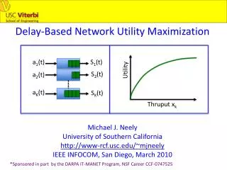
Delay-Based Network Utility Maximization. a 1 (t). S 1 (t). S 2 ( t). a 2 (t). Utility. a K ( t ). S K ( t ). Thruput x k. Michael J. Neely University of Southern California http://www-rcf.usc.edu/~mjneely IEEE INFOCOM, San Diego, March 2010.

Delay-Based Network Utility Maximization
E N D
Presentation Transcript
Delay-Based Network Utility Maximization a1(t) S1(t) S2(t) a2(t) Utility aK(t) SK(t) Thruputxk Michael J. Neely University of Southern California http://www-rcf.usc.edu/~mjneely IEEE INFOCOM, San Diego, March 2010 *Sponsored in part by the DARPA IT-MANET Program, NSF Career CCF-0747525
ak(t) Ψk(x(t), S(t)) • Network Model: • 1-Hop Network with K Queues--- (Q1(t), …, QK(t)) • Slotted time, t in {0, 1, 2, … } • S(t) = (S1(t), …, SK(t)) = “Channel State Vector” (i.i.d. over slots) • x(t) =(x1(t), …,xK(t)) = “Transmission Decision Vector” • a(t) = (a1(t), …, aK(t)) = “Packet Arrival Vector” (i.i.d. over slots) • Fixed Length Packets: a(t), x(t) are 0/1 vectors. • Arrival Rates: E{a(t)} = (λ1, …, λK). • Reliability is a Function of Transmission Decision: • Observe S(t) every slot. Choose 0/1 transmission vector x(t). • Pr[Success on link k | x(t), S(t)] = Ψk(x(t), S(t))
ak(t) Ψk(x(t), S(t)) Delay = 1 Delay = 2 Delay = 4 Queue k: Hk(t) = 4 Dropsk(t) • Packet Dropping: • We can decide to drop packets at any time. • Packets that fail in transmission can either be retransmitted • or dropped. • Thruput on channel k = yk = λk – drop rate on channel k • Delay-Based Control: • Stamp Head-of-Line (HOL) Packets with their Delays Hk(t). • Utility Maximization Objective: • Maximize: g1( y1 ) + g2( y2 ) + … + gK( yK) where gk(y) are concave, non-decreasing utility functions
Prior work on Stochastic Network Optimization: • Stability: (“Max-Weight” = “Min-Lyapunov-Drift”) • Tassiulas, Ephremides[1992, 1993] (Minimize drift Δ(t)) • Kahale, Wright [1997] • Andrews et. al. [2001] • Neely, Modiano, Rohrs [2003, 2005] • Kobayashi, Caire, Gesbert [2005] • Joint Stability and Utility Optimization: • Neely, Modiano [2003, 2005] (Minimize Δ(t) + V*Penalty(t)) • Georgiadis, Neely, Tassiulas [2006] • Stolyar [2005] (Primal-Dual “Fluid Model” analysis) • Special case of “Infinitely Backlogged Sources”: • Agrawal, Subramanian [2002], Kushner, Whiting [2002] • Eryilmaz, Srikant [2005], Lin, Shroff [2004] All of these references use queue backlog as weights!
Alternative “Delay-Based” Rules that use HOL Delays • as weights are known only for Network Stability: • Mekkittikul, McKeown [1996] • Shakkottai, Stolyar [2002] • Andrews, Kumaran, Ramanan,Stolyar, Vijaykumar, Whiting [2004] Our work fills the gap by developing a Delay-Based Rule for Maximizing Network Utility Subject to Stability. Utility Ψk(x(t), S(t)) ak(t) Thruputxk Delay = 1 Delay = 2 Delay = 4 Dropsk(t)
Challenges: • Prior “Drift-Plus-Penalty” Algorithm Admit/Drops Packets • Immediately when New Packets Arrive: Δ(t) + V*Penalty(t). • This does not directly Affect the HOL Values! • Tricky Correlation Issues between HOL sizes and Decisions! • Key Ideas for this paper: • Queue all packets. Admit/Drop only at HOL. • Use “Drift-Plus-Penalty” with a different queue structure • Use a “concavely extended utility function” • Advantages of Delay-Based Approach: • Provides “Delay-Fairness.” Queue-Based Rules can • leave loner packets stranded. • Provides Worst Case Delay Guarantees. • Disadvantage: Must know (λ1, …, λK) to implement.
Concavely Extending a Utility Function: gk(yk) fk(yk) slope = ηk slope = ηk yk yk 0 0 -1 1 1 Function gk(yk): Defined over 0 ≤ yk ≤ 1 Function fk(yk): Defined over -1 ≤ yk ≤ 1
Auxiliary Variables and Thruput Variables: yk(t) = λk – Dropsk(t) Time Avg: yk= λk – Dk θk(t), choose s.t. -1 ≤ θk(t) ≤ 1 Time Avg: θk Transformed Stochastic Net Optimization Problem: Maximize: f1( θ1) + f2( θ2) + … + fK( θK) Subject to: (1) E{Qk} < infinity , for all k in {1, …, K} (2) yk ≥ θk , for all k in {1, …, K} (3) -1 ≤ θk(t) ≤ 1 , for all t (4) yk, θk are time averages achievable on the network
Auxiliary Variables and Thruput Variables: yk(t) = λk – Dropsk(t) Time Avg: yk= λk – Dk θk(t), choose s.t. -1 ≤ θk(t) ≤ 1 Time Avg: θk Transformed Stochastic Net Optimization Problem: Maximize: f1( θ1) + f2( θ2) + … + fK( θK) Subject to: (1) E{Qk} < infinity , for all k in {1, …, K} (2) yk ≥ θk , for all k in {1, …, K} (3) -1 ≤ θk(t) ≤ 1 , for all t (4) yk, θk are time averages achievable on the network
Virtual Queue Zk(t) for enforcing constraint (2): Zk(t) θk(t) yk(t) = λk – Dropsk(t) Transformed Stochastic Net Optimization Problem: Maximize: f1( θ1) + f2( θ2) + … + fK( θK) Subject to: (1) E{Qk} < infinity , for all k in {1, …, K} (2) yk ≥ θk , for all k in {1, …, K} (3) -1 ≤ θk(t) ≤ 1 , for all t (4) yk, θk are time averages achievable on the network
Head-of-Line Delay Update Equation (Queue k): Hk(t+1) = 1{k full}(t) max[Hk(t) + 1 – (μk(t)+Dk(t))Tk(t), 0] + 1{k empty}(t) Ak(t) Inter-Arrival Time Tk(t) Service Drops Lyapunov Function: L(t) = (1/2)[H1(t)2 + … + HK(t)2] + (1/2)[Z1(t)2 + … + ZK(t)2] • Drift-Plus-Penalty Approach: • Observe {H1(t), …, HK(t)}, {Z1(t),…,ZK(t)}, {S1(t), …, SK(t)} • Take action to minimize: • Δ(t) – V [f1(θ1(t)) + ... + fK(θK(t))]
Δ(t) – V [f1(θ1(t)) + ... + fL(θL(t))] Resulting Algorithm: (Aux Variables) Each k observes Zk(t). Choose θk(t)to: Maximize : V f(θk(t)) – Zk(t)θk(t) Subject to: -1 ≤ θk(t) ≤ 1 2) (Transmission) Observe S(t), H(t), Z(t). Choose x(t) to: Maximize : xk(t) min[Hk(t), Zk(t)] Ψk(x(t),S(t)) Subject to: (x1(t),…, xK(t)) a 0/1 vector 3) (Packet Dropping) For each queue k with HOL packet that was not successfully transmitted, drop iffZk(t)≤Hk(t). 4) (Update Virtual and Actual Queues) Σk
Focus on Auxiliary Variable Update: Choose θk(t)to: Maximize : V f(θk(t)) – Zk(t)θk(t) Subject to: -1 ≤ θk(t) ≤ 1 Zk(t) < Vηk Zk(t) θk(t) yk(t) = λk – Dropsk(t) -1 1 Key Lemma: If Zk(t) > Vηk, then… …the above chooses θk(t) = -1 …hence, Zk(t) cannot increase on that slot: = -1 ≥ -1 [This is why we concavely extended the utility function over -1 ≤ y ≤ 1 ]
Focus on Auxiliary Variable Update: Choose θk(t)to: Maximize : V f(θk(t)) – Zk(t)θk(t) Subject to: -1 ≤ θk(t) ≤ 1 Zk(t) > Vηk Zk(t) θk(t) yk(t) = λk – Dropsk(t) -1 1 Key Lemma: If Zk(t) > Vηk, then… …the above chooses θk(t) = -1 …hence, Zk(t) cannot increase on that slot: = -1 ≥ -1 [This is why we concavely extended the utility function over -1 ≤ y ≤ 1 ]
Concluding Theorem: Implementing the above algorithm for any parameter V>0, we have… Delay: Worst Case Delay in Queue k ≤ Vηk + 2 slots. Total Utility Satisfies: g1( y1 ) + … + gK( yK ) ≥ g1( y1*) + … + gK( yK*) – B/V Achieved Utility Optimal Utility Utility Delay V V
Concluding Theorem: Implementing the above algorithm for any parameter V>0, we have… Delay: Worst Case Delay in Queue k ≤ Vηk + 2 slots. Total Utility Satisfies: g1( y1 ) + … + gK( yK ) ≥ g1( y1*) + … + gK( yK*) – B/V Achieved Utility Optimal Utility Utility Delay V V
Concluding Theorem: Implementing the above algorithm for any parameter V>0, we have… Delay: Worst Case Delay in Queue k ≤ Vηk + 2 slots. Total Utility Satisfies: g1( y1 ) + … + gK( yK ) ≥ g1( y1*) + … + gK( yK*) – B/V Achieved Utility Optimal Utility Utility Delay V V
Concluding Theorem: Implementing the above algorithm for any parameter V>0, we have… Delay: Worst Case Delay in Queue k ≤ Vηk + 2 slots. Total Utility Satisfies: g1( y1 ) + … + gK( yK ) ≥ g1( y1*) + … + gK( yK*) – B/V Achieved Utility Optimal Utility Utility Delay V V
Concluding Theorem: Implementing the above algorithm for any parameter V>0, we have… Delay: Worst Case Delay in Queue k ≤ Vηk + 2 slots. Total Utility Satisfies: g1( y1 ) + … + gK( yK ) ≥ g1( y1*) + … + gK( yK*) – B/V Achieved Utility Optimal Utility Utility Delay V V
Concluding Theorem: Implementing the above algorithm for any parameter V>0, we have… Delay: Worst Case Delay in Queue k ≤ Vηk + 2 slots. Total Utility Satisfies: g1( y1 ) + … + gK( yK ) ≥ g1( y1*) + … + gK( yK*) – B/V Achieved Utility Optimal Utility Utility Delay V V
Concluding Theorem: Implementing the above algorithm for any parameter V>0, we have… Delay: Worst Case Delay in Queue k ≤ Vηk + 2 slots. Total Utility Satisfies: g1( y1 ) + … + gK( yK ) ≥ g1( y1*) + … + gK( yK*) – B/V Achieved Utility Optimal Utility Utility Delay V V
Concluding Theorem: Implementing the above algorithm for any parameter V>0, we have… Delay: Worst Case Delay in Queue k ≤ Vηk + 2 slots. Total Utility Satisfies: g1( y1 ) + … + gK( yK ) ≥ g1( y1*) + … + gK( yK*) – B/V Achieved Utility Optimal Utility Utility Delay V V
Example Utility Function gk( y ) = log( 1 + ηky ) This approximates “proportionally fair” log-utility when ηk is large. The log-utility log( y ) has a singularity at y=0, and so is not always a good choice of utility function. Utility Delay V V