Image Processing for cDNA Microarray Data

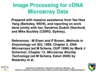
1. Image Processing for cDNA Microarray Data Prepared with massive assistance from Yee Hwa Yang (Berkeley, WEHI), and reporting on work done jointly with her, Sandrine Dudoit (Stanford) and Mike Buckley (CSIRO, Sydney). References : M Eisen and P Brown, Methods inEnzymology vol 303, 1999; Chapter 2, DNA Microarrays (ed M Schena, OUP 1999) by Mack J Schermer; Chapter 13, Microarray Biochip Technology (ed M Schena, Eaton 2000) by Basarsky et al.

2. Scanner Process A/D Convertor Laser PMT Dye Electrons Signal Photons excitation amplification Filtering Time-space averaging

3. GenePix 4000a Microarray Scanner Protocol 1. Turn on scanner. 2. Slide scanner door open. Insert chip hyp side down and clip chip holder easily around the slide 3 Set PMTs to 600 in both 635nm (Cy3) and 532 (Cy5) channels. 4. Perform low resolution “PREVIEW SCAN” to determine location of spots and initial hyb intensities 5. Once scan location determined, draw a “SCAN AREA” marquis around the array 6. Perform quick visual inspection of hyb and make initial adjustments to PMTs 7. For gene expression hybs, raise or lower the red and green PMTs to achieve color balance 8. Before you perform your data scan, change “LINES TO AVERAGE” to 2. 9. Perform a high-resolution “DATA-SCAN”……(ctd)

4. GenePix 4000a Microarray Scanner Protocol, ctd 10. Observe the histograms and make adjustments to PMTs. 11. Once the PMT level has been set so that the Intensity Ratio is near 1.00 perform a “DATA SCAN” over “SCAN AREA” and save the results. 12. To save your image, select “SAVE IMAGES”. 13. Save as type=Multi-image TIFF files. 14. Once scanned and saved, you are ready to assign spot identities and calculate results. Note: For us, normalization is performed later during data analysis, see next lecture.

5. Scanner PMT Pinhole Detector lens Laser Beam-splitter Objective Lens Dye Glass Slide

6. How to adjust for PMT? Very weak Cy3Cy5 1 600 600 2 650 600 3 650 650 4 700 650 5 650 700 6 700 700 7 750 750 saturated

7. After normalisation In addition, the ranking of the genes stays pretty much the same.

8. Practical Problems 1 • Comet Tails • Likely caused by insufficiently rapid immersion of the slides in the succinic anhydride blocking solution.

9. Practical Problems 2

10. Practical Problems 3 High Background • 2 likely causes: • Insufficient blocking. • Precipitation of the labeled probe. Weak Signals

11. Practical Problems 4 Spot overlap: Likely cause: too much rehydration during post - processing.

12. Practical Problems 5 Dust

13. Steps in Images Processing 1. Addressing: locate centers 2. Segmentation: classification of pixels either as signal or background. using seeded region growing). 3. Information extraction: for each spot of the array, calculates signal intensity pairs, background and quality measures.

14. Steps in Image Processing 3. Information Extraction • Spot Intensities • mean (pixel intensities). • median (pixel intensities). • Pixel variation (IQR of log (pixel intensities). • Background values • Local • Morphological opening • Constant (global) • None • Quality Information Signal Background

15. Addressing This is the process of assigning coordinates to each of the spots. Automating this part of the procedure permits high throughput analysis. 4 by 4 grids 19 by 21 spots per grid

16. Addressing Registration Registration

17. Problems in automatic addressing Misregistration of the red and green channels Rotation of the array in the image Skew in the array Rotation

18. Segmentation methods • Fixed circles • Adaptive Circle • Adaptive Shape • Edge detection. • Seeded Region Growing. (R. Adams and L. Bishof (1994) :Regions grow outwards from the seed points preferentially according to the difference between a pixel’s value and the running mean of values in an adjoining region. • Histogram Methods • Adaptive threshold.

19. Examples of algorithms and software implementation

20. Limitation of fixed circle method SRG Fixed Circle

21. Limitation of circular segmentation • Small spot • Not circular Results from SRG

22. Information Extraction • Spot Intensities • mean (pixel intensities). • median (pixel intensities). • Background values • Local • Morphological opening • Constant (global) • None • Quality Information Take the average

23. Local Backgrounds

24. Information • Quality • Area • Circularity • Signal to Noise ratio

25. Quality Measurements • Array • Correlation between spot intensities. • Percentage of spots with no signals. • Distribution of spot signal area. • Spot • Signal / Noise ratio. • Variation in pixel intensities. • Identification of “bad spot” (spots with no signal). • Ratio (2 spots combined) • Circularity

26. Quality of Array • Distribution of areas. • - Judge by eye • - Look at variation. (e.g, SD) • Cy5 area • mean 59 • median 57 • SD 24.34 • Cy3 area • mean 57 • median 56 • SD 20.67

27. Does the image analysis matter? Spot.nbg Spot.morph Spot.valley ScanAlyze

28. Background makes a difference Background method Segmentation method Exp1 Exp2 S.nbg 6 6 Gp.nbg 7 6 SA.nbg 6 6 No background QA.fix.nbg 7 6 QA.hist.nbg 7 6 QA.adp.nbg 14 14 S.valley 17 21 GP 11 11 Local surrounding SA 12 14 QA.fix 18 23 QA.hist 9 8 QA.adp 27 26 Others S.morph 9 9 S.const 14 14 Medians of the SD of log2(R/G) for 8 replicated spots multiplied by 100 and rounded to the nearest integer.