Design system with Bode
Design system with Bode. Hany Ferdinando Dept. of Electrical Eng. Petra Christian University. General Overview. Bode vs Root Locus design Information from open-loop freq. response Lead and lag compensator. Bode vs Root Locus.


Design system with Bode
E N D
Presentation Transcript
Design system with Bode Hany Ferdinando Dept. of Electrical Eng. Petra Christian University
General Overview • Bode vs Root Locus design • Information from open-loop freq. response • Lead and lag compensator Design System with Bode - Hany Ferdinando
Bode vs Root Locus • Root Locus method gives direct information on the transient response of the closed-loop system • Bode gives indirect information • In control system, the transient response is important. For Bode, it is represented indirectly as phase and gain margin, resonant peak magnitude, gain crossover, static error constant Design System with Bode - Hany Ferdinando
Open-loop Freq. Response • Low-freq. region indicates the steady-state behavior of the closed-loop system • Medium-freq. region indicates the relative stability • High-freq. region indicates the complexity of the system Design System with Bode - Hany Ferdinando
Lead and Lag Compensator • Lead Compensator: • It yields an improvement in transient response and small change in steady-state accuracy • It may attenuate high-freq. noise effect • Lag Compensator: • It yields an improvement in steady-state accuracy • It suppresses the effects of high-freq. noise signal Design System with Bode - Hany Ferdinando
Lead Compensator (0 < a < 1) The minimal value of a is limited by the construction of lead compensator. Usually, it is taken to be about 0.05 Design System with Bode - Hany Ferdinando
Lead Compensator • Define Kca = K then then • With gain K, draw the Bode diagram and evaluate the phase margin Determine gain K to satisfy the requirement on the given static error constant Design System with Bode - Hany Ferdinando
Lead Compensator • Determine the phase-lead angle to be added to the system (fm), add additional 5-12o to it • Use to determine the attenuation factor a. Find wc in G1(s) as |G1(s)| = -20 log(1/√a) and wc is 1/(√aT) • Find zero (1/T) and pole (1/aT) Design System with Bode - Hany Ferdinando
Lead Compensator • Calculate Kc = K/a • Check the gain margin to be sure it is satisfactory Design System with Bode - Hany Ferdinando
Lead Compensator - example • It is desired that the Kv is 20/s • Phase margin 50o • Gain margin at least 10 dB Design System with Bode - Hany Ferdinando
Lead Compensator - example K = 10 Design System with Bode - Hany Ferdinando
Lead Compensator - example Design System with Bode - Hany Ferdinando
Lead Compensator - example • Gain margin is infinity, the system requires gain margin at least 10 dB. • Phase margin is 18o, the system requires 50o, therefore there is additional 32o for phase margin • It is necessary to add 32o with 5-12o as explained before…it is chosen 5o 37o Design System with Bode - Hany Ferdinando
Lead Compensator - example • Sin 37o = 0.602, then a = 0.25 • |G1(s)| = -20 log (1/√a) wc = 8.83 rad/s new crossover freq. Design System with Bode - Hany Ferdinando
Lead Compensator - example • wc = 1/(√aT), then 1/T = wc√a = 4.415 zero = 4.415 • Pole = 1/(aT) = wc/√a = 17.66 • Kc = K/a = 10/0.25 = 40 Design System with Bode - Hany Ferdinando
Lead Compensator - example Design System with Bode - Hany Ferdinando
Lead Compensator - example clear; K = 10; num = 4; den = [1 2 0]; margin(K*num,den) [Gm,Pm] = margin(K*num,den) new_Pm = 50 - Pm + 5; new_Pm_rad = new_Pm*pi/180; alpha = (1 - sin(new_Pm_rad))/(1 + sin(new_Pm_rad)) Wc = 8.83; zero = Wc*sqrt(alpha); pole = Wc/sqrt(alpha); Kc = K/alpha; figure; margin(conv(4*Kc,[1 zero]),conv([1 2 0],[1 pole])) Clear variable Gain from Kv Original system Plot margin Get Gm & Pm New Pm in deg New Pm in rad alpha From calculation Get zero & pole Compensator gain Plot final result Design System with Bode - Hany Ferdinando
Lag Compensator (b > 1) With b > 1, its pole is closer to the origin than its zero is Design System with Bode - Hany Ferdinando
Lag Compensator • Assume Kcb = K Calculate gain K for required static error constant or you can draw it in Bode diagram Design System with Bode - Hany Ferdinando
Lag Compensator • if the phase margin of KG(s) does not satisfy the specification, calculate fm! It is fm = 180 – required_phase_margin (don’t forget to add 5-12 to the required phase margin). Find wc for the new fm! • Choose w = 1/T (zero of the compensator) 1 octave to 1 decade below wc. Design System with Bode - Hany Ferdinando
Lag Compensator • At wc, determine the attenuation to bring the magnitude curve down to 0 dB. This attenuation is equal to -20 log (b). From this point, we can calculate the pole, 1/(bT) • Calculate the gain Kc as K/b Design System with Bode - Hany Ferdinando
Lag Compensator - example • It is desired that the Kv is 5/s • Phase margin 40o • Gain margin at least 10 dB Design System with Bode - Hany Ferdinando
Lag Compensator - example K = Kcb With Kv = 5, K = 5 Design System with Bode - Hany Ferdinando
Lag Compensation - example Design System with Bode - Hany Ferdinando
Lag Compensation - example • The required phase margin is 40o, therefore, fm = -180o + 40o + 10o = -130o • Angle of G1(s) is -130o, wc = 0.49 rad/s • w = 1/T = 0.2wc = 0.098 rad/s • At wc, the attenuation to bring down the magnitude curve to 0 dB is -18.9878 dB (rounded to -19 dB) • From -20log(b) = -19, b is 8.9125 Design System with Bode - Hany Ferdinando
Lag Compensation - example • Pole of the compensator is 1/(bT), with 1/T = 0.098, the pole is 0.011 • Kc = K/b, and Kc = 0.561 Design System with Bode - Hany Ferdinando
Lag Compensation - example K = 5; num = 1; den = conv([1 1 0],[0.5 1]); margin(K*num,den) [Gm,Pm] = margin(K*num,den); new_Pm = (-180 + 40 + 10)*pi/180; %rad wc = 0.49; att = -(20*log10(5/abs(i*wc*(i*wc+1)*(i*0.5*wc+1)))) beta = 10^(att/-20) zero = 0.2*wc pole = zero/beta Kc = K/beta Gain Plot margin Get gain and phase margin Find new phase margin Design System with Bode - Hany Ferdinando