Desired Bode plot shape
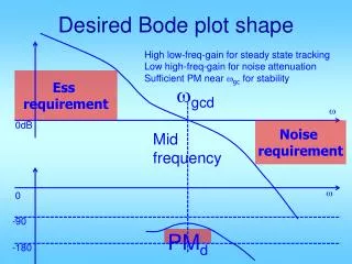
Desired Bode plot shape. High low- freq -gain for steady state tracking Low high- freq -gain for noise attenuation Sufficient PM near w gc for stability. Ess requirement. w gcd. w. 0dB. Noise requirement. Mid frequency. w. 0. -90. PM d. -180. Desired Bode plot shape.

Desired Bode plot shape
E N D
Presentation Transcript
Desired Bode plot shape High low-freq-gain for steady state tracking Low high-freq-gain for noise attenuation Sufficient PM near wgc for stability Ess requirement wgcd w 0dB Noise requirement Mid frequency w 0 -90 PMd -180
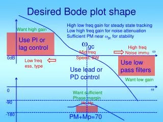
Desired Bode plot shape High low freq gain for steady state tracking Low high freq gain for noise attenuation Sufficient PM near wgc for stability Want high gain Use PI or lag control wgc w High freq 0dB Low freq Mid freq Use low pass filters Use lead or PD control Want low gain w 0 Want sufficient Phase margin -90 -180 PM+Mp=70
Controller design with Bode C(s) Gp(s) From specs: => desired Bode shape of Gol(s) Make Bode plot of Gp(s) Add C(s) to change Bode shape Get closed loop system Run step response, or sinusoidal response
Mr and BW are widely used Closed-loop phase resp. rarely used
Important relationships • Closed-loop BW are very close to wn • Open-loop gain cross over wgc ≈ (0.65~0.8)*wn, • When z <= 0.6, wr andwn are close • When z >= 0.7, no resonance • z determines phase margin and Mp: z 0.4 0.5 0.6 0.7 PM 44 53 61 67 deg ≈100z Mp 25 16 10 5 % PM+Mp ≈70
Mid frequency requirements • wgc is critically important • It is approximately equal to closed-loop BW • It is approximately equal to wn • Hence it determines tr, td directly • PM at wgc controls z • Mp 70 – PM • PM and wgc together controls s and wd • Determines ts, tp • Need wgc at the right frequency, and need sufficient PM at wgc
Low frequency requirements • Low freq gain slope and/or phase determines system type • Height of at low frequency determine error constants Kp, Kv, Ka • Which in turn determine ess • Need low frequency gain plot to have sufficient slope and sufficient height
High frequency requirements • Noise is always present in any system • Noise is rich in high frequency contents • To have better noise immunity, high frequency gain of system must be low • Need loop gain plot to have sufficient slope and sufficiently small value at high frequency
Overall Loop shaping strategy • Determine mid freq requirements • Speed/bandwidth wgc • Overshoot/resonance PMd • Use PD or lead to achieve PMd@ wgc • Use overall gain K to enforce wgc • PI or lag to improve steady state tracking • Use PI if type increase neede • Use lag if ess needs to be reduced • Use low pass filter to reduce high freq gain
Proportional controller design • Obtain open loop Bode plot • Convert design specs into Bode plot req. • Select KP based on requirements: • For improving ess: KP = Kp,v,a,des / Kp,v,a,act • For fixing Mp: select wgcd to be the freq at which PM is sufficient, and KP = 1/|G(jwgcd)| • For fixing speed: from td, tr, tp, or ts requirement, find out wn, let wgcd= (0.65~0.8)*wn and KP = 1/|G(jwgcd)|
clear all; n=[0 0 40]; d=[1 2 0]; figure(1); clf; margin(n,d); %proportional control design: figure(1); hold on; grid; V=axis; Mp = 10; %overshoot in percentage PMd = 70-Mp + 3; semilogx(V(1:2), [PMd-180 PMd-180],':r'); %get desired w_gc x=ginput(1); w_gcd = x(1); KP = 1/abs(evalfr(tf(n,d),j*w_gcd)); figure(2); margin(KP*n,d); figure(3); mystep(KP*n, d+KP*n);
KP/KD Bad for noise 20*log(KP) Place wgcd here
Could be a little less n=[0 0 1]; d=[0.02 0.3 1 0]; figure(1); clf; margin(n,d); Mp = 10/100; zeta = sqrt((log(Mp))^2/(pi^2+(log(Mp))^2)); PMd = zeta * 100 + 3; tr = 0.3; w_n=1.8/tr; w_gcd = w_n; PM = angle(polyval(n,j*w_gcd)/polyval(d,j*w_gcd)); phi = PMd*pi/180-PM; Td = tan(phi)/w_gcd; KP = 1/abs(polyval(n,j*w_gcd)/polyval(d,j*w_gcd)); KP = KP/sqrt(1+Td^2*w_gcd^2); KD=KP*Td; ngc = conv(n, [KD KP]); figure(2); margin(ngc,d); figure(3); mystep(ngc, d+ngc);
PD control design Variation • Restricted to using KP = 1 • Meet Mp requirement • Find wgc and PM • Find PMd • Let f = PMd – PM + (a few degrees) • Compute TD = tan(f)/wgcd • KP = 1; KD=KPTD
n=[0 0 5]; d=[0.02 0.3 1 0]; figure(1); clf; margin(n,d); Mp = 10/100; zeta = sqrt((log(Mp))^2/(pi^2+(log(Mp))^2)); PMd = zeta * 100 + 18; [GM,PM,wgc,wpc]=margin(n,d); phi = (PMd-PM)*pi/180; Td = tan(phi)/wgc; Kp=1; Kd=Kp*Td; ngc = conv(n, [Kd Kp]); figure(2); margin(ngc,d); figure(3); stepchar(ngc, d+ngc);
Example C(s) G(s) Want: maximum overshoot <= 10% rise time <= 0.3 sec Can use Lead or PD
Could be a little less n=[0 0 1]; d=[0.02 0.3 1 0]; figure(1); clf; margin(n,d); Mp = 10; %overshoot in percentage PMd = 70 – Mp + 3; tr = 0.3; w_n=1.8/tr; w_gcd = w_n; PM = angle(polyval(n,j*w_gcd)/polyval(d,j*w_gcd)); phi = PMd*pi/180-PM; Td = tan(phi)/w_gcd; KP = 1/abs(polyval(n,j*w_gcd)/polyval(d,j*w_gcd)); KP = KP/sqrt(1+Td^2*w_gcd^2); KD=KP*Td; ngc = conv(n, [KD KP]); figure(2); margin(ngc,d); figure(3); mystep(ngc, d+ngc);
Variation • Restricted to using KP = 1 • Meet Mp requirement • Find wgc and PM • Find PMd • Let f = PMd – PM + (a few degrees) • Compute TD = tan(f)/wgcd • KP = 1; KD=KPTD
KP=5; n=KP*[0 0 1]; d=[0.02 0.3 1 0]; figure(1); clf; margin(n,d); figure(3); stepchar(n, d+n);
KP=5; n=KP*[0 0 1]; d=[0.02 0.3 1 0]; figure(1); clf; margin(n,d); Mp = 10; PMd = 70 – Mp + 10; [GM,PM,wgc,wpc]=margin(n,d); phi = (PMd-PM)*pi/180; Td = tan(phi)/wgc; KP=1; KD=KP*Td; ngc = conv(n, [KD KP]); figure(2); margin(ngc,d); figure(3); stepchar(ngc, d+ngc);
KP=5; n=KP*[0 0 1]; d=[0.02 0.3 1 0]; figure(1); clf; margin(n,d); Mp = 10; PMd = 70 – Mp + 18; [GM,PM,wgc,wpc]=margin(n,d); phi = (PMd-PM)*pi/180; Td = tan(phi)/wgc; KP=1; KD=KP*Td; ngc = conv(n, [KD KP]); figure(2); margin(ngc,d); figure(3); stepchar(ngc, d+ngc);
plead zlead 20log(Kzlead/plead) Goal: select z and p so that max phase lead is at desired wgc and max phase lead = PM defficiency!
Lead Design • From specs => PMd and wgcd • From plant, draw Bode plot • Find PMhave = 180 + angle(G(jwgcd) • DPM = PMd - PMhave + a few degrees • Choose a=plead/zlead so that fmax = DPM and it happens at wgcd
Lead design example • Plant transfer function is given by: • n=[50000]; d=[1 60 500 0]; • Desired design specifications are: • Step response overshoot <= 16% • Closed-loop system BW>=20;
n=[50000]; d=[1 60 500 0]; G=tf(n,d); figure(1); margin(G); Mp_d = 16/100; zeta_d =0.5; % or calculate from Mp_d PMd = 100*zeta_d + 3; BW_d=20; w_gcd = BW_d*0.7; Gwgc=evalfr(G, j*w_gcd); PM = pi+angle(Gwgc); phimax= PMd*pi/180-PM; alpha=(1+sin(phimax))/(1-sin(phimax)); zlead= w_gcd/sqrt(alpha); plead=w_gcd*sqrt(alpha); K=sqrt(alpha)/abs(Gwgc); ngc = conv(n, K*[1 zlead]); dgc = conv(d, [1 plead]); figure(1); hold on; margin(ngc,dgc); hold off; [ncl,dcl]=feedback(ngc,dgc,1,1); figure(2); step(ncl,dcl);
After design Before design