Bode Plots in Frequency Domain Analysis
Learn about Bode plots, low and high frequency asymptotes, break frequencies, phase responses, and how to draw and interpret Bode plots in frequency domain analysis.

Bode Plots in Frequency Domain Analysis
E N D
Presentation Transcript
Bode Plot for G(s)=s+a • Let s=jω, G(jω)=jω+a= • At low frequencies, when ω approach zero, G(jω)≈a The magnitude response in dB is 20log M=20log a, where , a constant from ω=0.01a to a. • At high frequencies, ω>>a, G(jω)≈ The magnitude response in dB is 20 log M=20 log a + 20 log =20 log ω, where , y=20x, straight line
We call the low frequency approximation and high frequency approximation with the term low frequency asymptote and high frequency asymptote respectively. • The frequency, a, is called the break frequency. • As for phase response, at low frequency , the phase=0o, at high frequency, phase=90o. • To draw the curve, start one decade (1/10) below the break frequency (0.1a) , draw a line of slope +45o/decade passing through 45o at the break frequency and continue to 90o at one decade above the break frequency (10a).
To normalize (s+a), we factor out a and form a[(s/a)+1]. • By defining a new frequency variable, s1=s/a, then the magnitude is divided by a to yield 0 dB at the break frequency. • The normalized and scaled function is (s1+1). • To obtain the original frequency response, the magnitude and frequency is multiplied by a.
Table 10.1Asymptotic and actual normalized and scaledfrequency response data for (s + a)
Figure 10.7Asymptotic and actual normalized and scaled magnitude response of (s+ a)
Figure 10.8Asymptotic and actual normalized and scaled phase response of (s + a)
Bode Plot for G(s)=1/(s+a) The function has a low frequency asymptote of 20log(1/a), when s approach zero. The Bode plot is constant until break frequency, a rad/s is reached. At high frequency asymptote, when s approach infinity,
Normalized and scaled Bode plots for a. G(s) = s; b. G(s) = 1/s;c. G(s) = (s + a); d. G(s) = 1/(s + a)
Draw the Bode Plots for the system shown below, G(s)=K(s+3)/[s(s+1)(s+2)] The break frequencies are at 1,2,3. The magnitude plot should begin a decade below the lowest break frequency and extend to a decade above the highest break frequency. Hence, we choose 0.1 rad to 100 rad for this plot. The effect of K is to move the magnitude curve up and down by the amount of 20log K. K has no effect on the phase curve. Let K=1 in this case.
Bode Plot for The straight line is twice the slope of a first order term which is 40dB/decade.
Bode asymptotes for normalized and scaled G(s) =a. magnitude;b. phase
In second order polynomial, ωn is the break frequency. • For normalization, we divide the magnitude by ωn2, and scale the frequency , dividing by ωn . Thus, • G(s1) has a low frequency asymptote at 0dB and a break frequency of 1 rad/s. • For the phase plot, it is at 0o at low frequencies and 180o at high frequencies. The phase plot increase at a rate of 90o/decade from 0.1 to 10 and passes through 90o at 1. • The error between the actual response and the asymptotic approximation of the second order polynomial can be great depending on the value of ζ. • The actual magnitude and phase for are:
Draw the Bode log-magnitude and phase plots of G(s) for an unity feedback system.
Exercise: • Draw the Bode log-magnitude and phase plots for the system below:
Exercise: Root Locus • Given a unity feedback system with the forward transfer function: • Sketch the root locus • Find the imaginary-axis crossing • Find Gain K at jω-axis crossing • Find the break-in point • Find the angle of departure from the upper plane complex pole