Using Statistics Sample Statistics as Estimators of Population Parameters Sampling Distributions
430 likes | 925 Vues
Using Statistics Sample Statistics as Estimators of Population Parameters Sampling Distributions Estimators and Their Properties Degrees of Freedom Using the Computer Summary and Review of Terms. 5. Sampling and Sampling Distributions.

Using Statistics Sample Statistics as Estimators of Population Parameters Sampling Distributions
E N D
Presentation Transcript
Using Statistics Sample Statistics as Estimators of Population Parameters Sampling Distributions Estimators and Their Properties Degrees of Freedom Using the Computer Summary and Review of Terms 5 Sampling and Sampling Distributions
Make generalizations about the characteristics of a population... On the basis of observations of a sample, a part of a population 5-1 Statistics is a Science of Inference • Statistical Inference: • Predict and forecast values of population parameters... • Test hypotheses about values of population parameters... • Make decisions... On basis of sample statisticsderived from limited and incomplete sample information
The Literary Digest Poll (1936) Unbiased Sample Unbiased, representative sample drawn at random from the entire population. Democrats Republicans Population Biased Sample Biased, unrepresentative sample drawn from people who have cars and/or telephones and/or read the Digest. People who have phones and/or cars and/or are Digest readers. Democrats Republicans Population
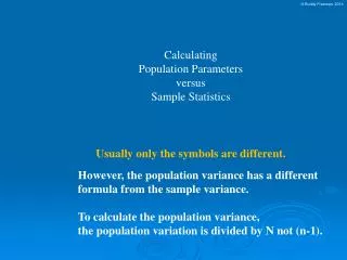
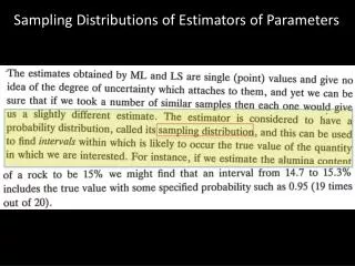
An estimatorof a population parameter is a sample statistic used to estimate or predict the population parameter. An estimate of a parameter is a particular numerical value of a sample statistic obtained through sampling. A point estimateis a single value used as an estimate of a population parameter. A sample statistic is a numerical measure of a summary characteristic of a sample. 5-2 Sample Statistics as Estimators of Population Parameters A population parameter is a numerical measure of a summary characteristic of a population.
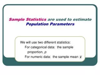
Estimators • The sample mean, X , is the most common estimator of the population mean, • The sample variance, s2, is the most common estimator of the population variance, 2. • The sample standard deviation, s, is the most common estimator of the population standard deviation, . • The sample proportion, p, is the most common estimator of the population proportion, p. ^
The population proportion is equal to the number of elements in the population belonging to the category of interest, divided by the total number of elements in the population: Population and Sample Proportions • The sample proportion is the number of elements in the sample belonging to the category of interest, divided by the sample size:
Population mean () Frequency distribution of the population X X X X X X X X X X X X X X X X X X Sample points Sample mean ( ) A Population Distribution, a Sample from a Population, and the Population and Sample Means
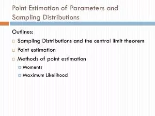
The sampling distribution of a statistic is the probability distribution of all possible values the statistic may assume, when computed from random samples of the same size, drawn from a specified population. The sampling distribution of Xis the probability distribution of all possible values the random variable may assume when a sample of size n is taken from a specified population. 5-3 Sampling Distributions (1)
U n i f o r m D i s t r i b u t i o n ( 1 , 8 ) 0 . 2 ) X ( 0 . 1 P 0 . 0 1 2 3 4 5 6 7 8 X Sampling Distributions (2) Uniform population of integers from 1 to 8: X P(X) XP(X) (X-x) (X-x)2 P(X)(X-x)2 1 0.125 0.125 -3.5 12.25 1.53125 2 0.125 0.250 -2.5 6.25 0.78125 3 0.125 0.375 -1.5 2.25 0.28125 4 0.125 0.500 -0.5 0.25 0.03125 5 0.125 0.625 0.5 0.25 0.03125 6 0.125 0.750 1.5 2.25 0.28125 7 0.125 0.875 2.5 6.25 0.78125 8 0.125 1.000 3.5 12.25 1.53125 1.000 4.500 5.25000 E(X) = = 4.5 V(X) = 2 = 5.25 SD(X) = = 2.2913
There are 8*8 = 64 different but equally-likely samples of size 2 that can be drawn (with replacement) from a uniform population of the integers from 1 to 8: Sampling Distributions (3) Each of these samples has a sample mean. For example, the mean of the sample (1,4) is 2.5, and the mean of the sample (8,4) is 6.
S a m p l i n g D i s t r i b u t i o n o f t h e M e a n 0 . 1 0 ) X ( P 0 . 0 5 0 . 0 0 1 . 0 1 . 5 2 . 0 2 . 5 3 . 0 3 . 5 4 . 0 4 . 5 5 . 0 5 . 5 6 . 0 6 . 5 7 . 0 7 . 5 8 . 0 X = m = E ( X ) 4. 5 X = s = V ( X ) 2 2. 625 X = s = SD ( X ) 1 . 6202 X Sampling Distributions (4) The probability distribution of the sample mean is called the sampling distribution of the the sample mean. Sampling Distribution of the Mean X P(X) XP(X) X-X (X-X)2 P(X)(X-X)2 1.0 0.015625 0.015625 -3.5 12.25 0.191406 1.5 0.031250 0.046875 -3.0 9.00 0.281250 2.0 0.046875 0.093750 -2.5 6.25 0.292969 2.5 0.062500 0.156250 -2.0 4.00 0.250000 3.0 0.078125 0.234375 -1.5 2.25 0.175781 3.5 0.093750 0.328125 -1.0 1.00 0.093750 4.0 0.109375 0.437500 -0.5 0.25 0.027344 4.5 0.125000 0.562500 0.0 0.00 0.000000 5.0 0.109375 0.546875 0.5 0.25 0.027344 5.5 0.093750 0.515625 1.0 1.00 0.093750 6.0 0.078125 0.468750 1.5 2.25 0.175781 6.5 0.062500 0.406250 2.0 4.00 0.250000 7.0 0.046875 0.328125 2.5 6.25 0.292969 7.5 0.031250 0.234375 3.0 9.00 0.281250 8.0 0.015625 0.125000 3.5 12.25 0.191406 1.000000 4.500000 2.625000
Comparing the population distribution and the sampling distribution of the mean: The sampling distribution is more bell-shaped and symmetric. Both have the same center. The sampling distribution of the mean is more compact, with a smaller variance. U n i f o r m D i s t r i b u t i o n ( 1 , 8 ) 0 . 2 ) X ( 0 . 1 P 0 . 0 1 2 3 4 5 6 7 8 X S a m p l i n g D i s t r i b u t i o n o f t h e M e a n 0 . 1 0 ) X ( P 0 . 0 5 0 . 0 0 1 . 0 1 . 5 2 . 0 2 . 5 3 . 0 3 . 5 4 . 0 4 . 5 5 . 0 5 . 5 6 . 0 6 . 5 7 . 0 7 . 5 8 . 0 Properties of the Sampling Distribution of the Sample Mean X
Relationships between Population Parameters and the Sampling Distribution of the Sample Mean The expected value of the sample meanis equal to the population mean: The variance of the sample meanis equal to the population variance divided by the sample size: The standard deviation of the sample mean, known as the standard error of the mean, is equal to the population standard deviation divided by the square root of the sample size:
Sampling from a Normal Population When sampling from a normal population with mean and standard deviation , the sample mean, X, has a normal sampling distribution: This means that, as the sample size increases, the sampling distribution of the sample mean remains centered on the population mean, but becomes more compactly distributed around that population mean S a m p l i n g D i s t r i b u t i o n o f t h e S a m p l e M e a n 0 . 4 Sampling Distribution: n =16 0 . 3 Sampling Distribution: n =4 ) X 0 . 2 ( f Sampling Distribution: n =2 0 . 1 Normal population Normal population 0 . 0
n=5 0 . 2 5 0 . 2 0 0 . 1 5 0 . 1 0 0 . 0 5 0 . 0 0 X n=20 0 . 2 0 . 1 0 . 0 X Large n 0 . 4 0 . 3 0 . 2 0 . 1 0 . 0 - X The Central Limit Theorem When sampling from a population with mean and finite standard deviation , the sampling distribution of the sample mean will tend to a normal distribution with mean and standard deviation as the sample size becomes large (n >30). For “large enough” n: ) X ( P ) X ( P ) X ( f
Normal Uniform Skewed General Population n = 2 n = 30 X X X X The Central Limit Theorem Applies to Sampling Distributions from Any Population
The Central Limit Theorem (Example 5-1) Mercury makes a 2.4 liter V-6 engine, the Laser XRi, used in speedboats. The company’s engineers believe the engine delivers an average power of 220 horsepower and that the standard deviation of power delivered is 15 HP. A potential buyer intends to sample 100 engines (each engine is to be run a single time). What is the probability that the sample mean will be less than 217HP?
EPS Mean Distribution 25 20 15 10 Frequency 5 0 6.00 - 6.49 7.00 - 7.49 2.00 - 2.49 5.00 - 5.49 3.00 - 3.49 4.00 - 4.49 Range Excel Output (Example 5-2)
The t is a family of bell-shaped and symmetric distributions, one for each number of degree of freedom. The expected value of t is 0. The variance of t is greater than 1, but approaches 1 as the number of degrees of freedom increases. The t is flatter and has fatter tails than does the standard normal. The t distribution approaches a standard normal as the number of degrees of freedom increases Standard normal t, df=20 t, df=10 Student’s t Distribution If the population standard deviation, , is unknown, replace with the sample standard deviation, s. If the population is normal, the resulting statistic: has a t distribution with (n - 1) degrees of freedom.
n = 2 , p = 0 . 3 0 . 5 0 . 4 0 . 3 ) X ( P 0 . 2 0 . 1 0 . 0 0 1 2 X n=10,p=0.3 0 . 3 0 . 2 ) X ( P 0 . 1 0 . 0 0 1 2 3 4 5 6 7 8 9 1 0 X n = 1 5 , p = 0 . 3 0 . 2 ) X ( P 0 . 1 0 . 0 X 0 1 2 3 4 5 6 7 8 9 1 0 1 1 1 2 1 3 1 4 1 5 ^ p 7 15 10 15 15 15 0 15 1 15 2 15 3 15 4 15 5 15 6 15 8 15 9 15 11 15 12 15 13 15 14 15 The Sampling Distribution of the Sample Proportion, The sample proportion is the percentage of successes in n binomial trials. I t is the number of successes, X, divided by the number of trials, n. Sample proportion: As the sample size, n, increases, the sampling distribution of approaches a normal distribution with mean p and standard deviation
In recent years, convertible sports coupes have become very popular in Japan. Toyota is currently shipping Celicas to Los Angeles, where a customizer does a roof lift and ships them back to Japan. Suppose that 25% of all Japanese in a given income and lifestyle category are interested in buying Celica convertibles. A random sample of 100 Japanese consumers in the category of interest is to be selected. What is the probability that at least 20% of those in the sample will express an interest in a Celica convertible? = n 100 æ ö ç ÷ = p 0 . 25 - - p p . 20 p $ > = ç > ÷ P ( p 0 . 20 ) P $ ç ÷ - - p ( 1 p ) p ( 1 p ) è ø = = = np ( 100 )( 0 . 25 ) 25 E ( p ) $ n n æ ö ç ÷ - (. 25 )(. 75 ) p ( 1 p ) æ ö - - . 20 . 25 . 05 = = = 0 . 001875 V ( p ) ç ÷ $ ç ÷ = > = > P z P z n 100 è ø ç ÷ . 0433 (. 25 )(. 75 ) è ø - 100 p ( 1 p ) = = = 0 . 001875 0 . 04330127 SD ( p ) $ = > - = P ( z 1 . 15 ) 0 . 8749 n Sample Proportion (Example 5-3)
Desirable properties of estimators include: Unbiasedness Efficiency Consistency Sufficiency 5-4 Estimators and Their Properties An estimator of a population parameter is a sample statistic used to estimate the parameter. The most commonly-used estimator of the: Population Parameter Sample Statistic Mean () is the Mean (X) Variance (2) is the Variance (s2) Standard Deviation () is the Standard Deviation (s) Proportion (p) is the Proportion ( )
Unbiasedness An estimator is said to be unbiased if its expected value is equal to the population parameter it estimates. For example, E(X)=so the sample mean is an unbiased estimator of the population mean. Unbiasedness is an average or long-run property. The mean of any single sample will probably not equal the population mean, but the average of the means of repeated independent samples from a population will equal the population mean. Any systematic deviation of the estimator from the population parameter of interest is called a bias.
{ Bias An unbiased estimator is on target on average. A biasedestimator is off target on average. Unbiased and Biased Estimators
An efficientestimator is, on average, closer to the parameter being estimated.. An inefficient estimator is, on average, farther from the parameter being estimated. Efficiency An estimator is efficient if it has a relatively small variance (and standard deviation).
Consistency n = 100 n = 10 Consistency and Sufficiency An estimator is said to be consistent if its probability of being close to the parameter it estimates increases as the sample size increases. An estimator is said to be sufficient if it contains all the information in the data about the parameter it estimates.
Properties of the Sample Mean For a normal population, both the sample mean and sample median are unbiased estimators of the population mean, but the sample mean is both more efficient (because it has a smaller variance), and sufficient. Every observation in the sample is used in the calculation of the sample mean, but only the middle value is used to find the sample median. In general, the sample mean is the best estimator of the population mean. The sample mean is the most efficient unbiased estimator of the population mean. It is also a consistent estimator.
å - æ ö 2 ( x x ) = = s 2 2 E ( s ) E ç ÷ - ( n 1 ) è ø å - æ ö ( x x ) 2 < s 2 E ç ÷ n è ø Properties of the Sample Variance The sample variance(the sum of the squared deviations from the sample mean divided by (n-1)) is an unbiased estimatorof the population variance. In contrast, the average squared deviationfrom the sample mean is a biased(though consistent) estimator of the population variance.
Consider a sample of size n=4 containing the following data points: x1=10 x2=12 x3=16 x4=? and for which the sample mean is: Given the values of three data points and the sample mean, the value of the fourth data point can be determined: 5-5 Degrees of Freedom (1)
If only two data points and the sample mean are known: x1=10 x2=12 x3=? x4=? The values of the remaining two data points cannot be uniquely determined: Degrees of Freedom (2)
å - 2 ( x x ) = 2 s - ( n 1 ) Degrees of Freedom (3) The number of degrees of freedomis equal to the total number of measurements (these are not always raw data points), less the total number of restrictions on the measurements. A restriction is a quantity computed from the measurements. The sample mean is a restriction on the sample measurements, so after calculating the sample mean there are only (n-1) degrees of freedom remaining with which to calculate the sample variance. The sample variance is based on only (n-1) free data points:
Example 5-4 A company manager has a total budget of $150.000 to be completely allocated to four different projects. How many degrees of freedom does the manager have? x1 + x2 + x3 + x4 = 150,000 A fourth project’s budget can be determined from the total budget and the individual budgets of the other three. For example, if: x1=40,000 x2=30,000 x3=50,000 Then: x4=150,000-40,000-30,000-50,000=30,000 So there are (n-1)=3 degrees of freedom.
4 0 3 0 y c n e u 2 0 q e r F 1 0 0 0 . 2 5 0 . 3 0 0 . 3 5 0 . 4 0 0 . 4 5 0 . 5 0 0 . 5 5 0 . 6 0 0 . 6 5 0 . 7 0 0 . 7 5 C 1 1 Using the Computer Constructing a sampling distribution of the mean from a uniform population (n=10): MTB > random 200 c1-c10; SUBC> uniform 0 1. MTB > rmean c1-c10 c11 MTB > histo c11 Character Histogram Histogram of C11 N = 200 Midpoint Count 0.25 1 * 0.30 5 ***** 0.35 11 *********** 0.40 27 *************************** 0.45 36 ************************************ 0.50 40 **************************************** 0.55 34 ********************************** 0.60 21 ********************* 0.65 18 ****************** 0.70 6 ****** 0.75 1 *
Histogram of Sample Means 250 200 150 Frequency 100 50 0 1 2 3 4 5 6 7 8 9 10 11 12 13 14 15 Sample Means (Class Midpoints) Using the Computer Constructing a sampling distribution of the mean from a uniform population (n=10) using EXCEL (use RANDBETWEEN(0, 1) command to generate values to graph): CLASS MIDPOINT FREQUENCY 0.15 0 0.2 0 0.25 3 0.3 26 0.35 64 0.4 113 0.45 183 0.5 213 0.55 178 0.6 128 0.65 65 0.7 20 0.75 3 0.8 3 0.85 0 999