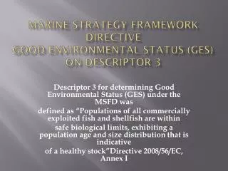
Descriptor 3

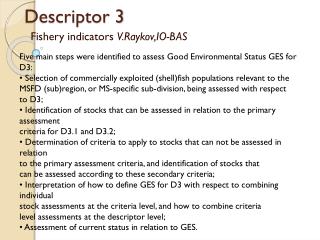
1. Descriptor 3 Five main steps were identified to assess Good Environmental Status GES for D3: • Selection of commercially exploited (shell)fish populations relevant to the MSFD (sub)region, or MS-specific sub-division, being assessed with respect to D3; • Identification of stocks that can be assessed in relation to the primary assessment criteria for D3.1 and D3.2; • Determination of criteria to apply to stocks that can not be assessed in relation to the primary assessment criteria, and identification of stocks that can be assessed according to these secondary criteria; • Interpretation of how to define GES for D3 with respect to combining individual stock assessments at the criteria level, and how to combine criteria level assessments at the descriptor level; • Assessment of current status in relation to GES. Fishery indicators V.Raykov,IO-BAS

2. The Choice • (1) Identification of the appropriate area • ; (2) Match of existing spatial units to that area; • (3) Choice of data • source; • (4) Choice of time period; • (5) Selection criteria.

3. Assessment • (1) all indicators with • reference levels, (2) not all reference levels, or (3) no reference levels. • For commercial populations that do not have full assessments scientific monitoring • surveys were identified as a potential data source for calculating some secondary indicators. • Three options for determining the current status from trend-based time series • were considered: (1) comparing the recent period mean with the long-term average • (2) comparing the current value of the indicator in relation to the historic mean • setting a threshold based on appropriate percentile of the Normal distribution; (3) detection • of trends.

4. GES • GES Interpretation 1: strict interpretation of the Commission Decision • where MSY reference levels are treated as a limit and thus all stocks must • meet the MSY requirement • • GES Interpretation 2: the MSY reference levels are considered as a target • and thus half the stocks must achieve the MSY requirement, and all stocks • must achieve precautionary reference levels • • GES Interpretation 3: the MSY reference levels are considered as a target • and stocks need to achieve this requirement on average. This average is • calculated accounting for the ‘distance’ individual stocks are above or below • the MSY reference level.

5. For the overall assessmentof Descriptor 3, three approaches were considered in the case studies: (1) noaggregation across criteria; (2) application of the one-out-all-out aggregation rule or“assessment by worst case”; or (3) application of weights for the different criteria. A higher proportion of assessed stocks increases the quality of the GES assessment; species/taxa for which no information is available decreases the quality; length of the time-series (with/without Reference levels);

6. Stocks for which analytical stock assessments are conducted F, SSB the populations for which only information from monitoring programs is available. Proportion of fish larger than the mean size of first sexual maturation ‘catch/biomass ratio’; Mean maximum length across all species found in research vessel surveys Biomass indices 95% percentile of the fish length distribution observed in research vessel surveys Size at first sexual maturation, which may reflect the extent of undesirable genetic effects of exploitation

7. Issues to be considered • Appropriate areas – divisions/subdivisions? • The time period over which the landings data are considered determines the relative importance of species or species groups; Threshold for inclusion of species – 1% but in Baltic Sea 0.5% as a threshold for salmon – important but with low catches;

8. Member States shall, when implementing their obligations under this Directive, take due • account of the fact that marine waters covered by their sovereignty or jurisdiction form an integral • part of the following marine regions: • (a) the Baltic Sea; • (b) the North-east Atlantic Ocean; • (c) the Mediterranean Sea; • (d) the Black Sea.

10. Fishing mortality

11. Fmsy,Fmax,F0.1 • Based on single species analysis (without ecosystem considerations; Predator-prey relationship);

12. SSB – single stock estimatins

13. Species covered by monitoring programs

14. What is GES?

17. Indicators calculation

18. Black Sea • Indicator calculations for BG waters

19. Biomass from scientific surveys

20. Catch, Fishing mortality Daskalov et al., 2012

21. Catch and biomass - TACs

22. Catch/Biomass ratio

23. Trends

24. Lmax (mean values) across all species caught in surveys

25. 95% Percentile from L

26. Sprat and turbot • Lmean Reference level for the given period of “healthy stock” condition • Holt (1958), Lopt – which assure max Y/R if all specimen were caught at the Lopt. • Froese et al. (2008) - Yield of the individuals reached Lopt, won’t affect negatively age structure of the population; • Froese and Sampang (2012) – the stock will have proportion of older individuals,if the mean length in the catch is within the interval: Lopt +/- 10%, i.e. 0.9 Lopt < Lmean < 1.1 Lopt. • For Loptcalculation the following equations is used: • logLopt = 1.0421 * logL∞ - 0.2742 (Froese and Binohlan, 2000). • where: L∞ - asymtoticlenght, Lopt – length at max Y/R

27. Classification of the state of Sprat population according to Lmean 7.20 cm < Lmean < 8.80 cm.

28. Long-term Lmean

29. Cumulative distribution of Length groups by years Cumulative contribution of TL=7cm varied 3.2-24.5%(max 2008,min 2010)

30. Age distribution

31. Turbot example (Black Sea)

32. Lmean Long term

33. Cumulative distribution of lenght

34. Thank you for the attention!