Download
1 / 22
220 likes | 339 Vues
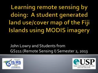
John Lowry and Students from GS211 (Remote Sensing I) Semester 2, 2013. Learning remote sensing by doing: A student generated land use/cover map of the Fiji Islands using MODIS imagery. Fiji Islands MODIS Image Jul 21, 2011 IOTD Aug 13, 2011.

E N D
John Lowry and Students from GS211 (Remote Sensing I) Semester 2, 2013 Learning remote sensing by doing: A student generated land use/cover map of the Fiji Islands using MODIS imagery
Fiji Islands MODIS Image Jul 21, 2011 IOTD Aug 13, 2011 NASA Earth Observatory Image of the Day http://earthobservatory.nasa.gov
Highlights of this presentation • Student learning more meaningful with “hands-on” learning through project-based activities • Remote sensing students at USP create first MODIS-based land use/cover map for Fiji Islands • Learning/teaching fundamentals of remote sensing accomplished using tools in ArcGIS & Google Earth
MODIS (Moderate Resolution Imaging Spectroradiometer) • Launched in 1999 • Terra & Aqua Satellites • 36 spectral bands • 250 m (bands 1 & 2) • 500 m (bands 3-7) • 1000 m (bands 8-36)
Primary Elements Color Tone (light-dark) Spatial Arrangement of Tone and Color Size Shape Texture Pattern Based on Analysis of Primary Elements Height Shadow Contextual Elements Site Association 10 Elements of Visual Interpretation
Classification Legend (Scheme) • Principal Vegetation Types of Fiji from Mueller-Dombois and Fosberg(1998) 10 Cloud Forest 20 Upland Rainforest 30 Lowland Rainforest 40 Mixed Dry Forest 50 Talasiga (grassland) 60 Mangrove forest and scrub 70 Plantation & Production 71 Hardwood Plantation 72 Softwood Plnatation 73 Coconut Palm 80 Anthropogentic Landscapes 81 Urban/Developed 82 Agriculture 90 Waterscapes 91 Water 92 Coral reef 100 Cloud cover
Vis. Interp. using Google Earth Talasiga (Grassland) Upland Rainforest Agriculture
Division of labour: 35 Mapping Zones Mapping zones created: Visually merged groups 2-3 Tikinas in ArcMap
Sample collection using Google Earth, guided with MODIS pixel grid Footprint created: Conversion Tools > From Raster > Raster to Polygon Converted to KML: Conversion Tools > To KML > Layer To KML
Sampling continued... • Each student: • Digitizes 25-40 polygons in mapping zone • Interprets homogenous land use/cover types that are 3+ footprint grid cells in size • Assigns numeric label to each sample polygon • Converted & Merged to ESRIGeodatabase Conversion to Geodatabase: Conversion Tools > From KML> KML to Layer (Batch) Then, Data Management > General > Merge
Reference Data (Sample Polygons) • Roughly 900 sample polygons total • After cleaning, 790 sample polygons total • Randomly divided: 50% Training 50% Accuracy Randomized division: Geostatistical Analyst > Utilities > Subset Features
Maximum Likelihood Classifier • Students experimented with EQUAL and SAMPLE prior probabilities • Produced classified maps and error matrices • Compared results visually & quantitatively Create signatures: Spatial Analyst > Multivariate > Create Signature Classification: Spatial Analysts > Multivariate >Maximum Likelihood Classifier
Accuracy Assess. MODIS Image Accuracy Assessment: Kappa Stats tool (Python script) from http://arcscripts.esri.com
Spectral Signatures for “natural” Vegetated Classes Create signatures: Spatial Analyst > Multivariate > Create Signature Graph in Excel
Use of Ancillary Data: Data Fusion Elevation: 100 m resolution Ave July Precip: 100 m resolution Resample to 500 m: Data management> raster > resample Normalized to same range as imagery: Spatial analyst > map algebra > raster calculator Create “Layer stack”: Data management > raster > raster processing > composite bands
Spectral Signatures for “natural” Vegetated Classes (w/ Ancillary Data) Create signatures: Spatial Analyst > Multivariate > Create Signature Graph in Excel
Accuracy Assess. W/Ancillary data Accuracy Assessment: Kappa Stats tool (Python script) from http://arcscripts.esri.com
Summary • Students experienced land use/cover classification project start-to-finish • Learned skills & understand theory by practice • Visual interpretation, sampling, spectral signatures, supervised classification, data fusion, accuracy assessment • 1:1,000,000* scale land use/cover map of Fiji Islands (2011) • Improvements with more training samples • Further experimentation, PCA, 250 m res. * Based on Tobler’s (1987) Rule of Thumb that map scale is 1,000 times double the pixel size (http://blogs.esri.com/esri/arcgis/2010/12/12/on-map-scale-and-raster-resolution/) Another useful website: http://www.scanex.ru/en/monitoring/default.asp?submenu=cartography&id=det