Download
1 / 22
220 likes | 298 Vues
Understanding genetic variation within and among subpopulations is crucial in population genetics. This study explores observed and expected heterozygosity levels across individuals and subpopulations to determine the overall genetic diversity in the total population. Various parameters are computed to assess the distribution of genetic variation and deviations from Hardy-Weinberg equilibrium. Discover how inbreeding coefficients and reduction in heterozygosity provide insights into population genetics. ###

E N D
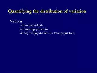
Quantifying the distribution of variation Variation within individuals within subpopulations among subpopulations (in total population)
Quantifying the distribution of variation Variation within individuals within subpopulations among subpopulations (in total population)
Quantifying the distribution of variation I = individuals S = subpopulations T = total population H is observed heterozygosity (# heterozygotes/N) in a population HIis observed heterozygosity (# heterozygotes/N) averaged over individuals in all subpopulations HSis expected heterozygosity in each subpopulation if it was in H-W equilibrium, averaged across subpopulations HT is expected heterozygosity if subpopulations are combined as one population
Quantifying the distribution of variation I = individuals S = subpopulations T = total population H is observed heterozygosity (# heterozygotes/N) in a population HIis observed heterozygosity (# heterozygotes/N) averaged over individuals in all subpopulations HSis expected heterozygosity in each subpopulation if it was in H-W equilibrium, averaged across subpopulations HT is expected heterozygosity if subpopulations are combined as one population HT HS HS HS
Quantifying the distribution of variation HIobserved heterozygosity averaged over individuals in all subpopulations HSexpected heterozygosity in each subpopulation (if it was in H-W equilib.) averaged across subpopulations HTexpected heterozygosity if subpopulations are combined as one population AA AA Aa aa aa Aa Aa Aa Aa AA p 0.50.6 H 1/5 = 0.2 4/5 = 0.8
Quantifying the distribution of variation HIobserved heterozygosity averaged over individuals in all subpopulations HSexpected heterozygosity in each subpopulation (if it was in H-W equilib.) averaged across subpopulations HTexpected heterozygosity if subpopulations are combined as one population AA AA Aa aa aa Aa Aa Aa Aa AA p 0.5 0.6 H 1/5 = 0.2 4/5 = 0.8 HI (0.2 + 0.8)/2 = 0.5
Quantifying the distribution of variation HIobserved heterozygosity averaged over individuals in all subpopulations HSexpected heterozygosity in each subpopulation (if it was in H-W equilib.) averaged across subpopulations HTexpected heterozygosity if subpopulations are combined as one population AA AA Aa aa aa Aa Aa Aa Aa AA p 0.5 0.6 H 1/5 = 0.2 4/5 = 0.8 HI (0.2 + 0.8)/2 = 0.5 HS (av. of 2pq) 2 x 0.5 x 0.5 = 0.5 2 x 0.6 x 0.4 = 0.48 (0.5 + 0.48)/2 = 0.49 If all subpopulations were in H-W equilibrium, HI would = HS
Quantifying the distribution of variation HIobserved heterozygosity averaged over individuals in all subpopulations HSexpected heterozygosity in each subpopulation (if it was in H-W equilib.) averaged across subpopulations HTexpected heterozygosity if subpopulations are combined as one population AA AA Aa aa aa Aa Aa Aa Aa AA p 0.5 0.6 H 1/5 = 0.2 4/5 = 0.8 HI (0.2 + 0.8)/2 = 0.5 HS (av. of 2pq) 2 x 0.5 x 0.5 = 0.5 2 x 0.6 x 0.4 = 0.48 (0.5 + 0.48)/2 = 0.49 HT (2 x pav x qav) 2 x 0.55 x 0.45 = 0.495
Quantifying the distribution of variation HIobserved heterozygosity averaged over individuals in all subpopulations HSexpected heterozygosity in each subpopulation (if it was in H-W equilib.) averaged across subpopulations HTexpected heterozygosity if subpopulations are combined as one population AA AA Aa aa aa Aa Aa Aa Aa AA p 0.5 0.6 H 1/5 = 0.2 4/5 = 0.8 HI (0.2 + 0.8)/2 = 0.5 HS (av. of 2pq) 2 x 0.5 x 0.5 = 0.5 2 x 0.6 x 0.4 = 0.48 (0.5 + 0.48)/2 = 0.49 HT (2 x pav x qav) 2 x 0.55 x 0.45 = 0.495 If all subpopulations were the same, HS would = HT
HIobserved heterozygosity averaged over individuals in all subpopulations HSexpected heterozygosity in each subpopulation averaged across subpopulations HTexpected heterozygosity if subpopulations are combined as one population FIT – reduction in heterozygosity of individuals relative to whole population FIT = HT – HI HT
HIobserved heterozygosity averaged over individuals in all subpopulations HSexpected heterozygosity in each subpopulation averaged across subpopulations HTexpected heterozygosity if subpopulations are combined as one population FIT – reduction in heterozygosity of individuals relative to whole population FIT = HT – HI HT - any departure from single panmictic population will lead to significant value - used to detect departures from Hardy-Weinberg equilibrium in total population
HIobserved heterozygosity averaged over individuals in all subpopulations HSexpected heterozygosity in each subpopulation averaged across subpopulations HTexpected heterozygosity if subpopulations are combined as one population FIS - inbreeding coefficient of individual relative to its sub- population (change in H due to non-random mating) FIS = HS – HI HS
HIobserved heterozygosity averaged over individuals in all subpopulations HSexpected heterozygosity in each subpopulation averaged across subpopulations HTexpected heterozygosity if subpopulations are combined as one population FIS - inbreeding coefficient of individual relative to its sub- population FIS = HS – HI HS used to detect departures from Hardy-Weinberg equilibrium in "good" populations positive value = heterozygote deficiency (Wahlund effect) zero value = all sub-populations in Hardy-Weinberg equilibrium (random mating within subpopulations) negative value = heterozygote excess
HIobserved heterozygosity averaged over individuals in all subpopulations HSexpected heterozygosity in each subpopulation averaged across subpopulations HTexpected heterozygosity if subpopulations are combined as one population FST - inbreeding coefficient of sub-population relative to the whole population = fixation index FST = HT – HS HT
HIobserved heterozygosity averaged over individuals in all subpopulations HSexpected heterozygosity in each subpopulation averaged across subpopulations HTexpected heterozygosity if subpopulations are combined as one population FST - inbreeding coefficient of sub-population relative to the whole population = fixation index FST = HT – HS HT measures degree of population differentiation within species (always positive) 0.00 = sub-popns have same allele frequencies 0.05-0.15 = moderate differentiation 0.15-0.25 = great differentiation >0.25 = extremely different 1.0 = popns fixed for different alleles
Dispersal and gene flow Taxa (# species) Fst Amphibians (33) 0.32 Reptiles (22) 0.26 Mammals (57) 0.24 Fish (79) 0.14 Insects (46) 0.10 Birds (23) 0.05 Plants – animal poll. 0.22 Plants – wind poll. 0.10
Quantifying the distribution of variation HIobserved heterozygosity averaged over individuals in all subpopulations (# heterozygotes/ total N) HSexpected heterozygosity in each subpopulation (if it was in H-W equilib.) averaged across subpopulations (# heterozygotes/total N) HTexpected heterozygosity if subpopulations are combined as one population HI HS HT AA, AA, AA , AA BB, BB, BB, BB 0 0 0.5 AA, AB, AB, BB AA, AB,AB, BB 0.5 0.5 0.5 AB, AB, AB, AB AB, AB, AB, AB 1 0.5 0.5 AA, BB, BB, BB AB, AB, AA, BB 0.25 0.440.47
Quantifying the distribution of variation FIS - inbreeding coefficient of individual relative to its sub- population FIS = HS – HI HS positive value = heterozygote deficiency zero value = all sub-populations in Hardy-Weinberg equilibrium negative value = heterozygote excess HI HS HT FIS AA, AA, AA , AA BB, BB, BB, BB 0 0 0.5 0 AA, AB, AB, BB AA, AB,AB, BB 0.5 0.5 0.5 0 AB, AB, AB, AB AB, AB, AB, AB 1 0.5 0.5 -1 AA, BB, BB, BB AB, AB, AA, BB 0.25 0.440.47 0.43
9 populations examined at 21 loci FIS = 0.49 high level of inbreeding? dioecious – so likely due to clustering of relatives Pacific yew (Taxus brevifolia)
Quantifying the distribution of variation FIT - reduction in heterozygosity of individuals relative to whole population FIT = HT – HI HT used to detect departures from Hardy-Weinberg equilibrium in total population HI HS HT FIT AA, AA, AA , AA BB, BB, BB, BB 0 0 0.5 1 AA, AB, AB, BB AA, AB,AB, BB 0.5 0.5 0.5 0 AB, AB, AB, AB AB, AB, AB, AB 1 0.5 0.5 -1 AA, BB, BB, BB AB, AB, AA, BB 0.25 0.440.47 0.46
Quantifying the distribution of variation FST - inbreeding coefficient of sub-population relative to the whole population FST = HT – HS HT measures degree of population differentiation within species (always positive) HI HS HT FST AA, AA, AA , AA BB, BB, BB, BB 0 0 0.5 1 AA, AB, AB, BB AA, AB,AB, BB 0.5 0.5 0.5 0 AB, AB, AB, AB AB, AB, AB, AB 1 0.5 0.5 0 AA, BB, BB, BB AB, AB, AA, BB 0.25 0.440.47 0.07
9 populations examined at 21 loci FST = 0.078 Low to moderate level of population differentiation Pacific yew (Taxus brevifolia)