Quantifying the Bessel Beam
Quantifying the Bessel Beam. Josh Nelson. Motivation. Ultimately we want to understand the Bessel beam we send into fiber optics. Thus, we must quantify our Bessel beam using a fitting algorithm There is no already made one so it must coded. Before the code. Slicing Normalizing.

Quantifying the Bessel Beam
E N D
Presentation Transcript
Quantifying the Bessel Beam Josh Nelson
Motivation • Ultimately we want to understand the Bessel beam we send into fiber optics. • Thus, we must quantify our Bessel beam using a fitting algorithm • There is no already made one so it must coded
Before the code • Slicing • Normalizing
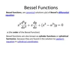
Code Basics • We want a model of the form: • c0*J0(A0*x) + c1*J1(A1*x) + … + c9*J9(A9*x) + F • 21 total constants: c0 – c9, A0 – A9, F • Restrictions: constants less than or equal to one. • So we must find the correct 21 constants! How?
The Loop • Steps: • Define all different combinations of Bessel Functions at 0.1 step sizes for coefficients • Take first combination and find intensity for all residual x-points in data • Find the difference between each residual intensity and square value
The Loop • Steps (cont): • Add all differences up and that gives total difference (or error) for Bessel function with those coefficients • Repeat for all combinations of Bessel Functions • Bessel function with the smallest difference is the best fit of the data
Problem • The number of calculations done is the number of steps for each coefficient to the power of the number of coefficients. • number of steps for each coefficient = 10 • number of coefficients = 21 • Number of calculations = 10^21
Problem • How long does that take to calculate? • 10^5 calculations = 20 minutes • So: • (10^5)/(10^21) = (20 min)/time • So time = 20*10^16 minutes • Or time = 380,517,503,805.2 years • What does this mean?
Solution… maybe • Loop functions seperately: • c0, A, F 6. c5, G, F • c1, B, F 7. c6, H, F • c2, C, F 8. c7, I, F • c3, D, F 9. c8, K, F • c4, E, F 10. c9, L, F
Solution… maybe • Each loop now has 10^3 calculations and takes about 2 seconds. • This gives a nice fit in about 20 seconds. • We can redo this same process starting with the new coefficients and refine the fit.
Possible Problem • Finding Local Minimum instead of Global Minimum
Future • Adding code for fitting at finer resolutions • Completely restarting if this turns out to just be a local minimum.


