Download
1 / 78
820 likes | 992 Vues
Use of Kalman filters in time and frequency analysis John Davis 1st May 2011. Overview of Talk. Simple example of Kalman filter Discuss components and operation of filter Models of clock and time transfer noise and deterministic properties

E N D
Use of Kalman filters in time and frequency analysis John Davis 1st May 2011
Overview of Talk • Simple example of Kalman filter • Discuss components and operation of filter • Models of clock and time transfer noise and deterministic properties • Examples of use of Kalman filter in time and frequency
Predictors, Filters and Smoothing Algorithms • Predictor: predicts parameter values ahead of current measurements • Filter: estimates parameter values using current and previous measurements • Smoothing Algorithm: estimates parameter values using future, current and previous measurements
What is a Kalman Filter ? • A Kalman filter is an optimal recursive data processing algorithm • The Kalman filter incorporates all information that can be provided to it. It processes all available measurements, regardless of their precision, to estimate the current value of the variables of interest • Computationally efficient due to its recursive structure • Assumes that variables being estimated are time dependent • Linear Algebra application
Operation of Kalman Filter • Provides an estimate of the current parameters using current measurements and previous parameter estimates • Should provide a close to optimal estimate if the models used in the filter match the physical situation • World is full of badly designed Kalman filters
What are the applications in time and frequency? • Analysis of time transfer / clock measurements where measurement noise is significant • Clock and time scale predictors • Clock ensemble algorithms • Estimating noise processes • Clock and UTC steering algorithms • GNSS applications
Five steps in the operation of a Kalman filter • (1) State Vector propagation • (2) Parameter Covariance Matrix propagation • (3) Compute Kalman Gain • (4) State Vector update • (5) Parameter Covariance Matrix update
Components of the Kalman Filter (1) State vector x • Contains required parameters. These parameters usually contain deterministic and stochastic components. • Normally include: time offset, normalised frequency offset, and linear frequency drift between two clocks or timescales. • State vector components may also include: Markov processes where we have memory within noise processes and also components of periodic instabilities
Components of the Kalman Filter (2) State Propagation Matrix F(t) • Matrix used to extrapolate the deterministic characteristics of the state vector from time t to t+t
Steps in the operation of the Kalman Filter Step 1: State vector propagation from iteration n-1 to n • Estimate of the state vector at iteration n not including measurement n. State propagation matrix calculated for time spacing t Estimate of the state vector at iteration n-1 including measurement n-1.
Components of the Kalman Filter (3) Parameter Covariance Matrix P • Contains estimates of the uncertainty and correlation between uncertainties of state vector components. Based on information supplied to the Kalman filter. Not obtained from measurements. Process Covariance Matrix Q(t) • Matrix describing instabilities of components of the state vector, e.g. clock noise, time transfer noise moving from time t to t+t Noise parameters s • Parameters used to determine the elements of the process covariance matrix, describe individual noise processes.
Steps in the operation of the Kalman Filter Step 2: Parameter covariance matrix propagation from iteration n-1 to n Parameter covariance matrix, at iteration n-1 including measurement n-1 State propagation matrix and transpose calculated for time spacing t Parameter covariance matrix, at iteration n not including measurement n Process covariance matrix
Components of the Kalman Filter (4) Design Matrix H • Matrix that relates the measurement vector and the state vector using y =H x Measurement Covariance Matrix R • Describes measurement noise, white but individual measurements may be correlated. May be removed. Kalman Gain K • Determines the weighting of current measurements and estimates from previous iteration. Computed by filter.
Steps in the operation of the Kalman Filter Step 3 :Kalman gain computation Parameter covariance matrix, at iteration n not including measurement n Design Matrix and Transpose Kalman Gain Measurement covariance matrix
Components of the Kalman Filter (5) Measurement Vector y • Vector containing measurements input during a single iteration of the filter Identity Matrix I
Steps in the operation of the Kalman Filter • Step 4 :State vector update • Estimate of the state vector at iteration n including and not including measurement n respectively. • Kalman Gain • Measurement Vector • Design Matrix
Steps in the operation of the Kalman Filter Step 5 :Parameter Covariance Matrix update • Kalman Gain • Design Matrix Parameter Covariance Matrix, at iteration n, including and not including measurement n respectively Identity Matrix
Steps in the operation of the Kalman Filter If Kalman gain is deliberately set sub-optimal, then use • Kalman Gain • Design Matrix Parameter Covariance Matrix, at iteration n, including and not including measurement n respectively Identity Matrix
Constructing a Kalman Filter: Lots to think about! • Choice of State Vector components • Choice of Noise Parameters • Choice of measurements • Description of measurement noise • Choice of Design Matrix • Choice of State Propagation Matrix • Initial set up conditions • Dealing with missing data • Testing out the filter • Computational methods
Initialising the Kalman Filter • Set the initial parameters to physically realistic values • If you have no information set diagonal values of Parameter Covariance Matrix high, filter will then give a high weight to the first measurement. • Set Parameters with known variances e.g. Markov components of Parameter Covariance Matrices to their steady state values. • Set Markov State Vector components and periodic elements to zero. • Elements of H,F(t),Q(t), R are pre-determined
Simulating Noise and Deterministic Processes • Use the same construction of state vector components x, state propagation matrix F(t), parameter covariance matrix P, process covariance matrix Q(t), design matrix H and measurement covariance matrix R. • Simulate all required data sets • Simulate “true” values of state vector for error analysis • May determine ADEV, HDEV, MDEV and TDEV statistics from parameter covariance matrix
Simulating Noise and Deterministic Processes Where = Process Covariance Matrix = State Vector at iteration n and n-1 respectively = State Propagation Matrix calculated for time spacing t = Vector of normal distribution noise of unity magnitude
Simulating Noise and Deterministic Processes Process Covariance Matrix at iterations n and n-1 respectively State Propagation Matrix and transpose computed at time spacing t. Process Covariance Matrix calculated at time spacing t
Simulating Noise and Deterministic Processes where Measurement Vector Design Matrix Measurement Covariance Matrix Vector of normal distribution noise of unity magnitude
ADEV, HDEV, and MDEV determined from Parameter Covariance Matrix and simulation z
Simulating Noise and Deterministic Processes • Test Kalman filter with a data set with same stochastic and deterministic properties as is expected by the Kalman filter. • Very near optimal performance of Kalman filter under these conditions.
Deterministic Properties • Linear frequency drift • Use three state vector components, time offset, normalised frequency offset and linear frequency drift
Markov Noise Process • White Noise • Random Walk Noise • Markov Noise • Flicker noise, combination of Markov processes with continuous range of relaxation parameters k • Markov noise processes and flicker noise have memory • Kalman filters tend to work very well with Markov noise processes • May only construct an approximation to flicker noise in a Kalman filter
Describing Measurement Noise • Kalman filter assumes measurement noise introduced via matrix R is white • Time transfer noise e.g TWSTFT and GNSS noise is often far from white • Add extra components to state vector to describe non white noise, particularly useful if noise has “memory” e.g. flicker phase noise • NPL has not had any problems in not using a measurement noise matrix R
Simulated FPM Noise -10 x 10 Flicker Phase Modulation 2 1.5 1 0.5 0 Time Offset -0.5 -1 -1.5 -2 -2.5 0 5 10 15 20 MJD
Clock Noise • White Frequency Modulation and Random Walk Frequency Modulation easy to include as single noise parameters. • Flicker Frequency Modulation may be modelled as linear combination of Integrated Markov Noise Parameters