Download
1 / 43
430 likes | 602 Vues
Statistics for Health Research. Statistical Inference for more than two groups. Peter T. Donnan Professor of Epidemiology and Biostatistics. Tests to be covered. Chi-squared test One-way ANOVA Logrank test. Significance testing – general overview

E N D
Statistics for Health Research Statistical Inference for more than two groups Peter T. Donnan Professor of Epidemiology and Biostatistics
Tests to be covered Chi-squared test One-way ANOVA Logrank test
Significance testing – general overview • Define the null and alternative hypotheses under the study • Acquire data • Calculate the value of the test statistic • Compare the value of the test statistic to values from a known probability distribution • Interpret the p-value and draw conclusion
Categorical data > 2 groups Unordered categories – Nominal - Chi-squared test for association Ordered categories - Ordinal - Chi squared test for trend
Example Does the proportion of mothers developing pre-eclampsia vary by parity (birth order)?
Contingency table (r x c)
Null Hypotheses Null hypothesis: No association between pre-eclampsia and birth order Null hypothesis: There is no trend in pre-eclampsia with parity
Test of association Test of linear trend
Conclusions Strong association between pre-eclampsia and birth order (Χ2 = 15.42, p = 0.001) Significant linear trend in incidence of pre-eclampsia with parity (Χ2 = 15.03, p < 0.001) Note 3 degrees of freedom for association test and 1 df for test for trend
Contingency table (r x c)
Contingency Tables (r x c) Tables can be any size. For example SIMD deciles by parity would be a 10 x 4 table But with very large tables difficult to interpret tests of association Crosstabulations in SPSS can give Odds ratios as an option with row or column with two categories
Numerical data > 2 groups Compare means from several groups Single global test of difference in means Also test for linear trend 1-way analysis of variance (ANOVA)
Extend t-test to >2 groups i.e Analysis of Variance (ANOVA) Consider scores for contribution to energy intake from fat groups, milk groups and alcohol groups Does the mean score differ across the three categories of intake groups? Koh ET, Owen WL. Introduction to Nutrition and Health Research Kluwer Boston, 2000
One-Way ANOVA of scores Contributor to Energy Intake Fat Milk Alcohol n=6 Mean=4.22 n=6 Mean=2.01 n=6 Mean=0.167
One-Way ANOVA of Scores The null hypothesis (H0) is ‘there are no differences in mean score across the three groups’ Use SPSS One-Way ANOVA to carry out this test
Assumptions of 1-Way ANOVA 1. Standard deviations are similar 2. Test variable (scores) are approx. Normally distributed If assumptions are not met, use non-parametric equivalent Kruskal-Wallis test
Results of ANOVA ANOVA partitions variation into Within and Between group components Results in F-statistic – compared with values in F-tables F = 108.6, with 2 and 15 df, p<0.001
Results of ANOVA The groups differ significantly and it is clear the Fat group contributes most to energy score with a mean = 4.22 Further pair-wise comparisons can be made (3 possible) using multiple comparisons test e.g. Bonferroni
Example 2 Does income vary by highest level of education achieved?
Null Hypothesis and alternative H0: no difference in mean income by education level achieved H1: mean income varies with education level achieved
Assumptions of 1-Way ANOVA Standard deviations or variances are similar Test variable (income) are approx. Normally distributed If assumptions are not met, use non-parametric equivalent Kruskal-Wallis test
Table of Mean income for each level of educational achievement
Analysis of Variance Table F-test gives P < 0.001 showing significant difference between mean levels of education
Table of each pairwise comparison. Note lower income for ‘did not complete school’ to all other groups. All p-values adjusted for multiple comparisons
Summary of ANOVA ANOVA useful if number of groups with continuous summary in each SPSS does all pairwise group comparisons adjusted for multiple testing Note that ANOVA is just a form of linear regression – see later
Extending Kaplan-Meier and logrank test in SPSS You need to specify: Survival time – time from surgery (tfsurg) Status – Dead = 1, censored = 0 (dead) Factor – Duke’s stage at baseline (A, B, C, D, Unknown) Select compare factor and logrank Optionally select plot of survival
Select options to obtain plot and median survival Select Compare Factor to obtain logrank test Select linear trend for this test
Overall Comparisons Chi-Square df Sig. Log Rank (Mantel-Cox) 80.534 1 .000 The vector of trend weights is -2, -1, 0, 1, 2. This is the default. The test for trend in survival across Duke’s stage is highly significant
Interpret SPSS output Note the logrank statistic, degrees of freedom and statistical significance (p-value). Note in which direction survival is worst or best and back up visual information from the Kaplan-Meier plot with median survival and 95% confidence intervals from the output. Finally, interpret the results!
Output form Kaplan-Meier in SPSS Note that SPSS gives three possible tests: Logrank, Tarone-Ware and Breslow In general, logrank gives greater weight to later events compared to the other two tests. If all are similar quote logrank test. If different results, quote more than one test result
Editing SPSS output Note that everything in the SPSS output window can be copied and pasted into Word and Powerpoint. Double-clicking on plots also allows editing of the plot such as changing axes, colours, fonts, etc.
Diabetic patients LDL data Try carrying out extended Crosstabulations and ANOVA where appropriate in the LDL data… E.g. APOE genotype
Colorectal cancer patients: survival following surgery Try carrying out Kaplan-Meier plots and logrank tests for other factors such as WHO Functional Performance, smoking, etc…
Extending test to more than 2 groups Summary • Define H0 and H1 • Choosing the appropriate test according to type of variables • Interpret output carefully