Download
1 / 17
180 likes | 292 Vues
Lecture 4 Exposition of the Lagrange Method. This lecture is technical. Please read Chow, Dynamic Economics, chapters 1 and 2. Brief explanation of the Lagrange method for dynamic optimization– 3 steps. 1. Start with the constrained maximization problem max r(x,u) subject to x=f(u).

E N D
Lecture 4 Exposition of the Lagrange Method This lecture is technical. Please read Chow, Dynamic Economics, chapters 1 and 2.
Brief explanation of the Lagrange method for dynamic optimization– 3 steps • 1. Start with the constrained maximization problem max r(x,u) subject to x=f(u). • Set up the Lagrange expression • L = r(x,u) –λ[x-f(u)]. • Differentiate L with respect to x, u and λ to obtain three first-order conditions. • Solve these equations for the three variables.
step 2 - Generalize above procedure to many periods • Objective function is a weighted sum of r(x(t),u(t)) over time t. • Constraints are x(t+1) = f(x(t),u(t)). • We call x the state variable and u the control variable. • Set up the Lagrange expression • L = Σtβt{r(x(t),u(t)) –λt+1[x(t+1)- f(x(t),u(t))]} and differentiate to obtain first-order conditions to solve for the u’s and x’s.
Step 3 - stochastic • Model is xt+1 = f(xt, ut, εt), εt stochastic. • We now have an expectation operator in front of the previous objective function • L = E Σ1Tβt {r(xt ,ut) – λt+1[xt+1 - f(xt ,ut)]} • The first-order conditions can still be obtained by differentiation after the summation sign. • This summarizes all I know after 30 years of work on dynamic optimization.
Problems • Do problems 1 and 3 of Chapter 2 of Chow, Dynamic Economics