Some "Special" Functions

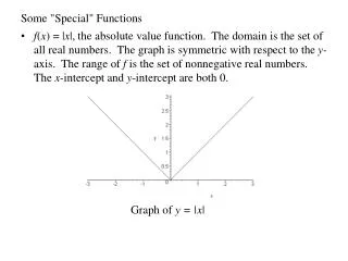
1. Some "Special" Functions • f(x) = |x|, the absolute value function. The domain is the set of all real numbers. The graph is symmetric with respect to the y-axis. The range of f is the set of nonnegative real numbers. The x-intercept and y-intercept are both 0. Graph of y = |x|

2. More "Special" Functions • f(x) = x2, the squaring function. The domain is the set of all real numbers. The graph is symmetric with respect to the y-axis. The range of f is the set of nonnegative real numbers. The x-intercept and y-intercept are both 0. Graph of y = x2

3. More "Special" Functions • f(x) = , the square root function. Since is not defined for x < 0, the domain is the set of nonnegative real numbers. The range of f is the set of nonnegative real numbers. The x-intercept and y-intercept are both 0. Graph of y =

4. More "Special" Functions • f(x) = x3, the cubic function. The domain is the set of all real numbers. The graph is symmetric with respect to the origin. The range of f is the set of all real numbers. The x-intercept and y-intercept are both 0. Graph of y = x3

5. Graphing Techniques--Vertical Shift • If p > 0, the graph of y = f(x) + p is the graph of y = f(x) shifted up p units. Similarly, the graph of y = f(x) –p is the graph of y = f(x) shifted down p units. y = x2 + 1 y = x2 y = x2 – 0.5

6. Graphing Techniques--Horizontal Shift • If p > 0, the graph of y = f(x – p) is the graph of y = f(x) shifted p units to the right. Similarly, the graph of y = f(x + p)is the graph of y = f(x) shifted p units to the left. y = x3 y = (x+2)3 y = (x–2)3

7. Graphing Techniques--Reflection • The graph of y =–f(x) is the reflection about the x-axis of the graph of y = f(x). The graph of y = f(–x) is the reflection about the y-axis of the graph of the graph of y = f(x). Reflection of y=|x–1| abouty-axis Reflection of y=x2 about x-axis

8. Graphing Techniques--Stretching and Shrinking • If k > 1, the graph of y =k f(x) is the graph of y = f(x) stretched vertically by k units. If 0 < k < 1, the graph of y = kf(x)is the graph of y = f(x) shrunk vertically by k units. y=2x2 y=x2 y=0.5x2

9. Piecewise Defined Functions • When a function is defined in different ways over different parts of its domain, it is said to be a piecewise-defined function. • Example. The price of a movie ticket changes from $5 to $8 at 5pm. We can write the cost C(t)of a ticket, in dollars, as the following piecewise-defined function of time t. • We recall that the absolute value function is also a piecewise-defined function.

10. Increasing and Decreasing Functions • If the graph of function f steadily rises as we go from left to right, we say that f is increasing. Similarly, if the graph of function f steadily falls as we go from left to right, we say that f is decreasing. • In general, a function may increase over some intervals, decrease over others, and remain constant in still other intervals. decreasing increasing

11. Linear and Quadratic Functions • The polynomial function is called a linear function. Its graph is a straight line. • The polynomial function of second degree is called a quadratic function. Its graph is in the shape of a parabola. For example, y = 2x2– 4x + 3

12. Summary of Graphs of Functions; We discussed • Graphs of the absolute value function, the squaring function, the square root function, and the cubic function • Vertical shift and horizontal shift • Reflection about the x-axis and about the y-axis • Vertical stretching and shrinking • Piecewise defined functions • Increasing and decreasing functions • Linear and quadratic functions

13. Linear Functions • The slope m of a line that is not vertical is given by where on the line. • Example. Find the slope of the line that passes through (5, 6) and (1, –2). • Slope measures the steepness of a line. On the line in the previous example, for every increase of 1 in x, we get an increase of 2 in y.

14. Properties of slope • Let m be the slope of a line. 1. When m > 0, the line is the graph of an increasing function. 2. When m < 0, the line is the graph of a decreasing function. 3. When m = 0, the line is the graph of a constant function. 4. Slope does not exist for a vertical line, and a vertical line is not the graph of a function. m = 3 m = –3 m = 1 m = –1 m = 1/2 m = –1/2

15. Equation of a line: Point-Slope Form • The equation is that of a line with slope m that passes through the point (x1, y1). • Example. Find an equation of the line that passes through the points (6, –2) and (–4, 3). First we calculate the slope m = –0.5. We let (x1, y1) = (6, –2), although we could have validly used the other point. The equation is:

16. Equation of a line: Slope-Intercept Form • The equation is that of a line with slope m and y-intercept b. • Example. Find an equation of the line that passes through the points (1, 2) and (0, 3). We calculate the slope as m = –1. Since we are given that the y-intercept = 3, the equation is:

17. Horizontal and Vertical Lines • The equation is that of the horizontal line through the point (a, b). The slope of a horizontal line is 0. • The equation is that of the vertical line through the point (a, b). A vertical line has undefined slope.

18. General First Degree Equation of a Line • The graph of the general first-degree equation is a line. • If A = 0, the graph is a horizontal line. • If B = 0, the graph is a vertical line. • Example. Convert x + 2y + 3 = 0 to slope-intercept form.

19. Parallel and Perpendicular Lines • Two lines with slopes m1 and m2 are parallel if and only if • Two lines with slopes m1 and m2 are perpendicular if and only if • Example. Given the line y = 3x – 2, find an equation of the line through (–5, 4) that is (a) parallel to the given line, (b) perpendicular to the given line (a) (b)

20. Linear Functions; We discussed • Slope of a line • Slope for increasing, decreasing, and constant linear functions • Point-slope form • Slope-intercept form • Horizontal and vertical lines • General first degree equation • Parallel and perpendicular lines