Forecasting Basic Concepts And Stationary Models
Forecasting Basic Concepts And Stationary Models. What is Forecasting?. Forecasting is the process of predicting the future. Forecasting is an integral part of almost all business enterprises including

Forecasting Basic Concepts And Stationary Models
E N D
Presentation Transcript
Forecasting Basic Concepts And Stationary Models
What is Forecasting? • Forecastingis the process of predicting the future. • Forecasting is an integral part of almost all business enterprises including • Manufacturing firms that forecast demand for their products, to schedule manpower and raw material allocation. • Service organizations that forecast customer arrival patterns to maintain adequate customer service. • Security analysts who forecast revenues, profits, and debt ratios, to make investment recommendations. • Firms that consider economic forecasts of indicators (housing starts, changes in gross national profit) before deciding on capital investments.
Benefits of Forecasting Good forecasts can lead to Reduced inventory costs Lower overall personnel costs and increased customer satisfaction A higher likelihood of making profitable financial decisions A reduced risk of untimely financial decisions
How Does One Prepare a Forecast? • The forecasting process can be based on: • Educated guess. • Expert opinions. • Past history of data values, known as a time series.
Components of a Time Series • Long-term Trend Effects • Long-term trend is typically modeled as a linear, quadratic or exponential. • A time series that does not exhibit any trend over time is a stationary model. • Seasonal Effects • When a predictable, repetitive pattern is observed, the time series is said to have seasonal effects. • Seasonal effects can be associated with calendar/climatic changes or tied to yearly, quarterly, monthly, etc. data • Cyclical Effects • An unanticipated “temporary” upturn or downturn that is not explained by seasonal effects are said to be cyclical effects. • Cyclical effects can result from changes in economic conditions. • Random Effects
Long Term Trend Cyclical Effects Recessions of Early 80’s and 90’s ExampleMotorhome Sales 1975-2000 Seasonal Effects Qtr 4 Lower than qtr 3 Qtr 3 Higher than qtr 2 Qtr 2 Higher than qtr 1 Qtr 1 Higher than qtr 4
Steps in the Time Series Forecasting Process • The goal of a time series forecast is to identify factors that canbe predicted. • This is a systematic approach involving the following steps. • Step 1: Hypothesize a form for the time series. • Collect historical data and graph the data vs. time. • Hypothesize and statistically verify a form for the time series. • Step 2: Select a forecasting technique from a set of possible methods for the form of the time series. • Statistically determine which method best forecasts the data. • Step 3: Prepare a forecast.
Stationary Forecasting Models • Assumptions for εt • independent • normally distributed • have a mean of 0 Value of the random error at time t Value of the time series at time t True stationary value of the time series • A stationary model is one that forecasts a constant time series value over time. • The general form of such a model is: yt = b0 + et
Determining if a Stationary Model Is Appropriate • Is theretrend? • Use Linear Regression -- Check the p-value for 1 • Is there seasonality? • Visually check of time series graph • Autocorrelation measures the relationship between the values of the time series every k periods; this is called autocorrelation of lag k. • There are tests for doing this, but we will just do a visual check. • Lag 7 autocorrelation indicates one week seasonality (daily data); lag 12 autocorrelation indicates 12-month seasonality (monthly data), etc. • Are there cyclical effects? • Visually check of time series graph.
Moving Averages • There are t observations: y1 (oldest), y2, y3, …, yt (most recent) • In stationary forecasting models, the forecast for the constant value, β0, for the next time period t+1, Ft+1, is the average (or a weighted average) of 1 or more of the immediately prior observations, yt, yt-1, etc. • Since the time series is stationary, this forecast for time period t+1, will be the forecast for all future periods: t+2, t+3, etc. • The forecast changes only after more data is collected.
Moving Average Methods • Last Period Ft+1 = yt • Use the last observed value of the time series • n period Moving Average Ft+1 = (yt + yt-1 + … + yt-n+1)/k • Average the last n observed values of the time series • n period Weighted Moving Average Ft+1 = wtyt + wt-1yt-1 + … wt-n+1yt-n+1 • Weight the last n observed values (the w’s sum to 1) • Exponential Smoothing*(*Discussed in another module) • All observations are weighted with decreasing weights
Example Galaxy Industries needs to forecast weekly demand for the next three weeks for its Yoho brand yoyo based on the past 52 week’s demand. If demand is deemed to be stationary, use: • Last Period Technique • 4-Period Moving Average Technique • 4-Period Weighted Moving Average Technique (.4, .3, .2, .1)
Determining if the Model Is Stationary No discernable seasonal or cyclical effects. • Graph the time series.
Using Regression to Test for Trend Select Regression from Data Analysis in Tools Menu
Using Regression to Test for Trend Demand Time Periods Where output is to begin
Is Linear Trend Present? High p-value = .71601 No indication of linear trend Stationary model is appropriate. • Check p-value for β1.
Forecasts • Since we have concluded that this is a stationary model, we can use moving average methods. Last Period: • Since model is stationary, F55 = F54 = F53 = 484 4 Period Moving Average: • Since model is stationary, F55 = F54 = F53 = 401 4 Period Weighted (.4, .3, .2, .1) Moving Average: • Since model is stationary, F55 = F54 = F53 = 441.3 F53 = y52 = 484 F53 = (y52 + y51 + y50 + y49)/4 = (484 + 482 + 393 + 245)/4 = 401 F53 = .4y52 + .3y51 + .2y50 + .1y49 = .4(484) + .3(482) + .2(393) + .1(245) = 441.3
EXCEL: Last Period =B2 Drag cell C3 down to cell C54 =C54 Drag cell C55 down to cell C56 Note: Rows 8-43 are hidden
Excel: Moving Average Forecast =Average(B2:B5) Drag cell C6 down to cell C54 =C54 Drag cell C55 down to cell C56 Note: Rows 8-43 are hidden
Excel: Weighted Moving Average =.4*B5+.3*B4+.2*B3+.1*B2 Drag cell C6 down to cell C54 =C54 Drag cell C55 down to cell C56 Note: Rows 8-43 are hidden
Review • Possible Factors in a Time Series Model • Trend, Seasonal, Cyclical, Random Effects • Determining if the Time Series is Stationary • No noticeable seasonal or cyclical effects on time series plot • Use Regression to test for β1 = 0 • High p-value (No trend – stationary) • Moving Average Forecasting Methods • Last Period, Moving Average, Weighted Moving Average, Exponential Smoothing • Forecasts for next period will be the forecasts for all future periods until additional time series values occur • Excel approach