Download

1 / 21
210 likes | 325 Vues
EEE515J1 ASICs and DIGITAL DESIGN Lecture 6: Data Processors and Control Units. Ian McCrum Room 5D03B Tel: 90 366364 voice mail on 6 th ring Email: IJ.McCrum@Ulster.ac.uk Web site: http://www.eej.ulst.ac.uk . Last changed 01/11/04@18:00. Designing Larger Digital Systems:.

E N D
EEE515J1ASICs and DIGITAL DESIGN Lecture 6: Data Processors and Control Units Ian McCrum Room 5D03B Tel: 90 366364 voice mail on 6th ring Email: IJ.McCrum@Ulster.ac.uk Web site: http://www.eej.ulst.ac.uk Last changed 01/11/04@18:00
Designing Larger Digital Systems: • We have seen how designing Finite state machines (FSMs) is relatively straightforward once the state diagram or design specification is drawn. • Together with combinational logic these design methods will stand you in good stead. • Of course there are problems that would be rather large or tedious to solve using these methods such as a system with a large number of inputs or one with a large variety of actions or steps to be performed. • We can modify the FSM approach. • Having one FSM send inputs and receive outputs from another FSM is a useful technique, such cascaded or coupled FSMs are found in real designs; • the design techniques used will depend on whether the two FSMs have synchronous clocks. • If not then the system is an asynchronous one and will use handshake and control to effect synchronisation between the machines. • We will not dwell (sic) on such machines here except to note that testing asynchronous systems is difficult, error prone and can give a design which is difficult to modify late in the design cycle.
The Algorithmic State Machine method • Other modifications to the basic FSM method might add memory such as stack or heap structures and have state machines route data to and from these memory structures. • A more general approach is described below. • Another alternative is to use a computer or microprocessor system and write software. • Actually a computer is just an instance of a digital system and the stored program concept on which its application is based is similar to the design method below so it should come as no surprise that if you can master the method below you will understand how computers actually work, and could even design your own CPU.
The ASM Method • Instead of concentrating on simply moving from state to state we can decompose our problem into a number of sections. • If we must process input data and can identify simple operations to be performed on the data then we can sequence and control the flow of data to and from each data processing block using FSM design methods. • Thus we partition our system into a “DATA PROCESSOR” and a “CONTROL LOGIC” section. • The data processor has functional blocks that “do something” to the incoming data or locally generated data such as a count of items processed. • A good design rule is that each functional block should do one thing and be easily described. It might be a counter, an added or comparator or shift register. It could even be a complete ALU. • The Control Logic sends control signals to each block and receives status signals or information about the data but not the data itself. Many choices can be made by the designer but as a rule this partition gives an easily designed, easily tested and easily modified system
External Inputs ( only a few and preferably synchronised to the system clock) Input Data CONTROL LOGIC Actually a FSM; receiving inputs and deciding what sequences of outputs to generate. Control Signals DATA PROCESSOR Simple blocks, each of which does a single, simple, easily expressed function. Status Signals Output Data The ASM Method An ALU or Arithmetic Logic Unit has typically 2 data inputs and a data output all 8 or 9 bits wide. It also has 3 or 4 inputs to indicate what to do. The 3 bit binary number 000…111 might specify F=A+B, A-B, B-A, A and B, A or B and maybe F=A, F=B and F=11111111
Example of ASM method • Averaging 16 numbers each of 8 bits in size • Method 1: use 8 adders to add 8 pairs of numbers, this gives 8 9 bit numbers (worst case) • Use 4 9-bit adders to give four 10 bit answers • Use 2 10 bit adders to give two 11 bit answers • Finally use a 11 bit adder giving a 12 bit answer, we can use a trick to “divide by 16” – simply use the 8 left most bits of the 12 bit number, akin to shifting right 4 bits, this is division by 2^4. • This is obviously most wasteful of space, but achieves a reasonably fast answer, 4 add-times. • Actually adders are slow, though there are a number of special techniques to speed up addition, c.f carry-lookahead-adders. • Clearly a more space efficient system would be to do the calculation the way humans would do it. Use a running total and add sequentially, I.e use one adder and pass the data through it one number at a time.
DATA IN S (START) 0 1 S ADD ADD ADDER CLEAR STROBE STROBE REGISTER 1 DATAVALID EQ16 DATAVALID 0 S1 S6 S0 S2 S3 S4 S5 COUNT CLEAR COUNTER (RESETABLE) COUNT EQ16 DETECT 16 CLOCK Example of ASM method State equations S0.D:= S0./s + S2 S1.D:= S0. S S2.D:= S5.EQ16 S3.D:= S1 + S6 S4.D:= S3 S5.D:= S4 S6.D:= S5./EQ16 Output equations CLEAR = S1 ADD = S3 STROBE = S5 COUNT = S6 DATAVALID = S2
Data out DATA VALID Data out Data out REQUEST STROBE 0 1 REQ STROBE 0 1 ack Data out STROBE Signals to the outside world • Several unanswered problems remain with the previous design • Exactly when the input arrives • The datavalid pulse is only available for a short time • It would be “better” ( “cheaper”?)to use countdown counter. • Often when doing an initial ASM design, the interface to the outside world (or the next machine in the chain)is not given much attention. • A typical, useful approach is to provide handshake lines to allow flow control. Thus ack RECEIVER driven, Wait for REQUEST I/p then o/p data, then o/p DATAVALID, often just a timed pulse , a low-high-low Sender driven, o/p data, then o/p strobe, keep it high until ack is seen from far end
strobe strobe clock ASM machines demand synchronous logic • Even simple latches are best driven in a synchronous manner, even though applying a “latch” or “strobe” signal to the clocks of a register ( e.g 8 D-type flip-flops) will work, a more testable circuit results if the master clock goes to every component. • Thus the D-types spend most of their time in a “held” state and only “load data” when the strobe signal is high • This is easily achieved by adding multiplexors
Using a CLOCK • The role of the clock is very important in the ASM method. • As has been said before, having everything synchronised to a single clock can ease testing and last minute design modifications. • In very large systems you will find systems that use two phase clocks where the rising edge is used by one section of a system and the next section uses the falling edge. • Or latches are provided to isolate adjacent sections. • Multiphase clocks exist, a 4 phase solution allows “the soldiers all to march in step”. • Very large fast systems will have problems routing a clock signal from one edge of a chip to the other and several solutions exist to fix this. • Often the designer will lay down the clock distribution network before adding other gates. • A matrix of equal delay buffers may allow distribution with a low timing skew across chip. • Also used today is local generation of the clock and a system of phase locking ( cf www.altera.com for a description of their DPLL cells). This can also allow the clock frequency off-chip to be much lower than the clock on the chip, the phase locking can be done at a sub multiple of the clock frequency. I first saw this on a Transputer chip were the chip internally worked at 20MHz but you only needed to supply the chip with a 5 Mhz oscillator. The PCB layout was less critical and the emitted RF noise was much less with this approach. You may be aware it is used a lot in modern PC CPU design, sometimes the internal clocks run at 3.5 times the external clocks!. ( cf www.tomshardwareguide.com )
Synchronous Control signals: • A key to initial ASM designs is to have very strict synchronisation. This rule has even prompted some TTL companies to bring out two versions of their chips; the 74163 and 74163A counters are identical except that the RESET action is synchronised on one version but asynchronous on the other. • Once you are familiar with the method and have a dozen designs under your belt you may relax this strict rule somewhat. • Chips such as counters and shift registers can undertake various control actions; the RESET, LOAD, PRESET, DIRECTION controls for a counter are all VERBS of ACTION. An important part of the method is to recognise that whilst your control logic may assert these control inputs they are NOT acted upon until the next clock pulse. Thus the ACTION is not taken until the clock pulse. This makes the design diagrams easier to follow.
The Design Method • There are two main steps both graphical in nature; a block diagram of the data processor and the ASM chart describing the sequence of data operations to be performed. Different problems sometimes lend themselves to applying these in different orders. The data processor is a block diagram or circuit diagram where each block is a simple functional circuit. As a guide each block should be available as a TTL chip but if you have little experience of the TTL family a further guide should be to ensure that it performs a single, easily explained task. Each block should be simple to design such as a combinational problem or a very simple FSM. • All control signals MUST be synchronous. Combinational circuits such as ADDERS might have a synchronous ADD control signal or you can just assume the answer pops out the bottom of the adder. You must ensure that the propagation delays of each data processor block do not cause problems; if these are all much faster than the clock then there will be no problem. It is possible to insert dummy states into the Control logic to wait for answers to appear, or we must complicate our system by adding status signals e.g “ADDER_COMPLETE”
The Design Method continued • The ASM chart is comprised of boxes of just three types. • It superficially resembles a programming flowchart. There is one crucial difference; Programming Flowcharts are read sequentially from the top of the page to the bottom, if there is only one CPU then this also represents the time behaviour of the program. • Obviously in a hardware circuit with a couple of counters the counting of one counter does not wait for the counting of another. Both pieces of hardware operate at the same time, concurrently. • In fact the different parts of the Data Processor in an ASM all operate at the same time. If we have a section of an ASM chart where a counter is told to count, an input is tested and an output is generated then these actions will all be scheduled to happen at the same time. • Of course it will take the next clock pulse to action the events. • Each “state” in an ASM chart has only one output box. • It may have a number of input testing boxes and output boxes conditional on some inputs but there must only be one main output box per state. • All arrows arriving at that state must go through this box. • We label the state by labelling that output box but be clear where the dotted lines that form the boundary of our state lie, see Figure 2 overleaf.
S0 0001 A <-A+1, R1 <- 0 0 1 E 1 F R2 <- 11111111 0 Figure 2: Different shapes of an ASM The Design Method continued • Note some texts will name the state inside a bubble shown as a dotted circle. Here I have listed the state S0, with a state code of 0001. (I will use one-hot codes for the state code but there is no reason why a more efficient code couldn’t be used) • When “in” state zero you are in all boxes inside the dotted line simulaneously! Depending on input conditions. Thus the single bit input “E” is tested at the same time as the single bit input “F” is tested, the PRESET or LOAD_ALL_ONES control signal of the 8 bit register R2 is asserted if E is high, it flickers if E flickers but of course we should try and use synchronous inputs where possible. The Adder ( or counter?) A is to increment and the RESET signal of R1 is asserted. • Maybe you see now why all control signals are only activated on a clock pulse. All these control signals are set or cleared but NO action takes place until the clock pulse arrives that will take the machine to its next state, down one of the three arrows exiting the box.
The Design Method continued • One of the consequences of this method means that if a test is activated instantly on entering a state then it is based on the old values of the inputs. • If the state alters an input then we must be most careful. If the conditional boxes above tested the counter/adder A then it would exit depending on the old value of A, despite A altering as we left the state. • It is a good idea not to test a signal in the same state as you attempt to alter it • It is easy to add “dummy” states (empty state boxes) to cause a one clock cycle delay and this can decouple the two effects. It is usually a good idea to avoid two tests within one state. • These rules or guidelines can be broken but adherence will increase the likelihood that the system will work!
Counting ‘1’s in a 16 bit word. The previous example was extremely abstract, a more typical application follows; we begin with an English description of the problem. “A system is needed that will count the number of ones in a 16 bit word. The design should be easily modified for a 32 bit word.” This is a nice example because, as in real life, there are many possible solutions, the good designer will reject all but one of these, the one that is picked will be for a good reason! Here we will adopt an ASM method to illustrate the design method. Speed of response or cost may push a real designer to different conclusions.
Register R1 containing word Large Combinational circuit. Register R1 containing word Solution 1b: create a 4 bit cell and iterate the answer. Adders will be needed to combine the four outputs and this will be a slower, but easier to design solution. Solution 1a The answer will be between zero and 16 inclusive. This needs 5 bits to represent it (00000…10000) Solution 2: Use a shift Register and counter. This will demonstrate the ASM method quite nicely. Note that the two solutions trade space and time. The pure combinational approach is fastest but largest. We will use a shift register and shift each bit out in turn; if it is a ‘1’ we will increment a counter. As is often the case we need to know when to stop. This could be done by having a loop counter keep track of how many shifts we had done, beginners usually set up a counter to go from zero ( or 1) to 16. This may be out by one and a comparator is needed. Experienced ASM designers ( and programmers) preload a counter with 15 and decrement to zero or find an alternative. Here we will use a clever trick to save time. By shifting zeros into our word as we shift our data out we can test for all zeros to exit our loop. In the case where there are few ones this may give an impressive speed advantage, at the disadvantage that the execution time of our machine varies according to the input data; that is not always allowed.
Simple Combinational circuit. ( NOR gate) Detects ALL_ZEROS SHIFT Register R1 containing word LOAD ‘1’ ‘1’ ‘1’ ‘1’ Counter COUNT LOAD Solution 2: Shift Register and adder… • This will demonstrate the ASM method quite nicely. Note that the two solutions trade space and time. The pure combinational approach is fastest but largest. • We will use a shift register and shift each bit out in turn; if it is a ‘1’ we will increment a counter. • As is often the case we need to know when to stop. This could be done by having a loop counter keep track of how many shifts we had done, beginners usually set up a counter to go from zero ( or 1) to 16. This may be out by one and a comparator is needed. • Experienced ASM designers ( and programmers) preload a counter with 15 and decrement to zero or find an alternative. • Here we will use a clever trick to save time. By shifting zeros into our word as we shift our data out we can test for all zeros to exit our loop. • In the case where there are few ones this may give an impressive speed advantage, at the disadvantage that the execution time of our machine varies according to the input data; that is not always allowed. Initial sketch of Data Processor
S Control Logic Implementing the ASM Chart below Simple Combinational circuit. ( NOR gate) Detects ALL_ZEROS SHIFT Register R1 containing word LOAD ‘1’ ‘1’ ‘1’ ‘1’ Counter COUNT LOAD D Q Figure 9: The Data Processor, one way of solving the problem, alternatively leave out the D-Type Flip-Flop. Not shown here is how the answer is read from the counter and how the input is wired up to the shift register’s parallel data inputs Solution 2: Shift Register and adder…
T0 INITIAL STATE 0 S 1 R1 INPUT (LOAD) R2 ‘1111’ (LOAD) T1 COUNT 1 0 Z T2 SHIFT T3 DUMMY STATE 1 0 E Solution 2: Shift Register and adder… The one-hot equations for this machine are as follows… T0.d = T0 * /S + T1 * Z T1.d = T3 * E + T0 * S T2.d = T1 * /Z + T3 * /E T3.d = T2 ; this causes a one clock delay between altering E and testing E. Also the control signals are LOAD = T0 * S COUNT = T1 SHIFT = T2
Try the tut questions! See the file ASMTUTS.pdf on the website The only “trick” to some of them is the use of a pipeline, a line of registers to allow access to older data… I’ll do a DSP pipeline design on the board, its not hard. Remember real ADCs will need to be given a SC control signal and will return an EOC status signal. These stand for START_CONVERSION and END_OF_CONVERSION.