Download
1 / 55
560 likes | 867 Vues
Introduction to SPSS for GHA Staff. Prof Gwilym Pryce: g@gpryce.com Tutors: George Vlachos, Christian Holz Lab notes based on material by John Malcolm. Plan:. A. Data Types 1. Variables 2. Constants B. Introduction to SPSS 1. SPSS Menu Bar 2. File Types C. Tabulating Data

E N D
Introduction to SPSS for GHA Staff Prof Gwilym Pryce: g@gpryce.com Tutors: George Vlachos, Christian Holz Lab notes based on material by John Malcolm
Plan: • A. Data Types • 1. Variables • 2. Constants • B. Introduction to SPSS • 1. SPSS Menu Bar • 2. File Types • C. Tabulating Data • 1. Categorical variables • 2. Continuous variables • D. Graphing Data • 1. Categorical variables • 2. Continuous variables
A. Data Types • 1. Variables • 2. Constants
1. What is a variable? • A measurement or quantity that can take on more than one value: • E.g. size of planet: varies from planet to planet • E.g. weight: varies from person to person • E.g. gender: varies from person to person • E.g. fear of crime:varies from person to person • E.g. income: varies from HH to HH • I.e. values vary across ‘individuals’ = the objects described by our data
Individuals = basic units of a data set whom we observe or experiment on in a controlled way • not necessary persons • (could be schools, organisations, countries, groups, policies, or objects such as cars or safety pins) • Variables = information that can vary across the individuals we observe • e.g. age, height, gender, income, exam scores, whether signed Nuclear Test Ban Treaty
Variable Type, for Coding Purposes:Variable View of the Data
Variable Type for Coding Purposes: • Available data types in SPSS are as follows: • Numeric – the default for new variables • Comma • Dot • Scientific Notation • Date • String
Numeric • A variable whose values are numbers. Values are displayed in standard numeric format. • The Data Editor accepts numeric values in standard format or in scientific notation. • Comma • A numeric variable whose values are displayed with commas delimiting every three places, and with the period as a decimal delimiter. • The Data Editor accepts numeric values for comma variables with or without commas, or in scientific notation. • Values cannot contain commas to the right of the decimal indicator.
Dot • A numeric variable whose values are displayed with periods delimiting every three places and with the comma as a decimal delimiter. • The Data Editor accepts numeric values for dot variables with or without periods, or in scientific notation. • Values cannot contain periods to the right of the decimal indicator. • Scientific notation • A numeric variable whose values are displayed with an imbedded E and a signed power-of-ten exponent. • The Data Editor accepts numeric values for such variables with or without an exponent. • The exponent can be preceded either by E or D with an optional sign, or by the sign alone--for example, 123, 1.23E2, 1.23D2, 1.23E+2, and even 1.23+2.
Date • A numeric variable whose values are displayed in one of several calendar-date or clock-time formats. Select a format from the list. You can enter dates with slashes, hyphens, periods, commas, or blank spaces as delimiters. The century range for two-digit year values is determined by your Options settings (from the Edit menu, choose Options and click the Data tab). • Custom currency • A numeric variable whose values are displayed in one of the custom currency formats that you have defined in the Currency tab of the Options dialog box. Defined custom currency characters cannot be used in data entry but are displayed in the Data Editor.
String • Values of a string variable are not numeric and therefore are not used in calculations. • They can contain any characters up to the defined length. • Uppercase and lowercase letters are considered distinct. • Also known as an alphanumeric variable.
Conceptual Approach to Variable Type: • Numeric = values are numbers that can be used in calculations. • String = Values are not numeric, and hence not used in calculations. • But can often be coded: I.e. transformed into a numerical variable: • e.g. If (LA = ‘Aberdeen’) X = 1. If (LA = ‘East Renfrewshire’) X = 2. etc.
Continuous vs Categorical • Continuous (or Scale or quantitative Variables) = data values are numeric values on an interval or ratio scale • (e.g., age, income). Scale variables must be numeric. • E.g. dimmer switch: brightness of light can be measured along a continuum from dark to full brightness • Categorical Variables = variables that have values which fall into two or more discrete categories • E.g. conventional light switch: either total darkness or full brightness, on or off. • Male or female, employment category, country of origin
Two types of Categorical variables: Ordinal & Nominal • Ordinal variables = Data values represent categories with some intrinsic order • (e.g., low, medium, high; strongly agree, agree, disagree, strongly disagree). • Ordinal variables can be either string (alphanumeric) or numeric values that represent distinct categories (e.g., 1=low, 2=medium, 3=high).
Ordinal variables: • Values fall within discrete but ordered categories • I.e. the sequence of categories has meaning • e.g. education categories: • 1 = primary • 2 = secondary • 3 = college • 4 = university undergraduate • 5 = university postgraduate masters • 6 = university postgraduate phd • e.g. 1= Very poor, 2= poor, 3=good, 4=very good
Nominal variables • Nominal Variables = Data values represent categories with no intrinsic order • sequence of categories is arbitary -- ordering has no meaning in and of itself: • e.g. country of origin: Wales, Scotland, Germany… • e.g. make of car: Ford, Vauxhall • e.g. job category • e.g. company division • Nominal variables can be either string (alphanumeric) or numeric values that represent distinct categories (e.g., 1=Male, 2=Female).
2. What is a constant? • A measurement or quantity that has only one value for all the objects described in our data • Also called a ‘scalar’ or ‘intercept’ or ‘parameter’ • E.g. speed of light in a vacuum: constant for all light transmissions • E.g. ratio of diameter to circumf.: constant for all circles • E.g. ave. increase in life expectancy: constant at 1 year pa since 1900 • E.g. Price elasticity of housing supply: assumed constant for a particular market
Often it is a constant that want to estimate: • we employ statistical techniques to estimate ‘parameters’ or ‘constants’ that summarise or link variables. • e.g. mean = ‘typical’ value of a variable = measure of central tendency • e.g. standard deviation = measure of the variability of a variable = measure of spread • e.g. correlation coefficient = measures the correlation between two variables • e.g. slope coefficients = how much y increases when x increases
Plan: • A. Data Types • 1. Variables • 2. Constants • B. Introduction to SPSS • 1. SPSS Menu Bar • 2. File Types • C. Tabulating Data • 1. Categorical variables • 2. Continuous variables • D. Graphing Data • 1. Categorical variables • 2. Continuous variables
B. Introduction to SPSS1. SPSS Menu Bar • When you first open SPSS, you will usually be presented with a blank Data View window • The Data View lists variables as columns and observations (also called “cases” or “individuals”) as rows • Data View without and with data looks like this…
B.2. File Types & SPSS Structure • If you try opening a new file (File, New), you will see that you are presented with five choices of file type. • These choices reflect the basic structure of SPSS: • Data • Syntax • Steep learning curve, but essential for larger projects • Backup • Record/checking • Re-use • Output • Graphs, tables, commands, error messages
SPSS Scripting Facility • The scripting facility allows you to automate tasks, including: • Automatically customize output in the Viewer. • Open and save data files. • Display and manipulate dialog boxes. • Run data transformations and statistical procedures using command syntax. • Export charts as graphic files in a number of formats.
Plan: • A. Data Types • 1. Variables • 2. Constants • B. Introduction to SPSS • 1. SPSS Menu Bar • 2. File Types • C. Tabulating Data • 1. Categorical variables • 2. Continuous variables • D. Graphing Data • 1. Categorical variables • 2. Continuous variables
C. Tabulating Data • 1. Categorical Data: Frequency Tables • E.g. Neighbourhood type (House Sales data) • Analyse, Descriptive Statistics, Frequencies
Categorical Data: Crosstabs (2-Way Tables) • E.g. Does Ethnic Minority Status affect job type? (Emplment data) • Analyse, Descriptive Statistics, Crosstabs
2. Scale Data • Scale or quantitative data: usually a measurement of size or quantity • not meaningful to report % or count • Not unless you break the variale into categories (& then it becomes categorical data!) • e.g. income bands = “grouped data” • Tables of raw data not much use unless only a few values...
Tables of Summary Statistics for Continuous Data: • Descriptives Function in SPSS: • E.g. House Sales data • On SPSS Menu Bar select: • Analyze, Descriptive Statistics, Descriptives
Explore Function in SPSS: • On SPSS Menu Bar select: • Analyze, Descriptive Statistics, Explore
Plan: • A. Data Types • 1. Variables • 2. Constants • B. Introduction to SPSS • 1. SPSS Menu Bar • 2. File Types • C. Tabulating Data • 1. Categorical variables • 2. Continuous variables • D. Graphing Data • 1. Categorical variables • 2. Continuous variables
D. Graphs of Variables: 1. Graphs of Categorical Data • Pie Charts • If all the categories sum to a meaningful total, then you can use a pie chart • Pie charts emphasise the differences in proportions between categories • OK for a single snapshot, but not very good for showing trends • would need to have a separate pie chart for each year
On SPSS Menu Bar select: • Graphs, Pie, Summaries for Groups of Cases
Bar Charts • can show either % or count • not very good for showing trends in more than one category
D. Graphs of Variables: 2. Graphs of Continuous Data • What are we interested in when describing data? • E.g. income: • Is income evenly spread? • Or are most people rich? • Or are most people poor? • Or are most reasonably well off? • This are all questions about the variable’s Distribution • We can represent the whole data set with one picture...
On SPSS Menu Bar select: • Graphs, Histogram, and select variable