Computing Suspended-Sediment Concentrations and Loads from In-Stream Turbidity and Streamflow Data
280 likes | 521 Vues
Computing Suspended-Sediment Concentrations and Loads from In-Stream Turbidity and Streamflow Data. Heather Bragg Oregon Water Science Center USGS Sediment Data Collection Techniques March 24-28,2014. PURPOSE. Provide overview

Computing Suspended-Sediment Concentrations and Loads from In-Stream Turbidity and Streamflow Data
E N D
Presentation Transcript
Computing Suspended-Sediment Concentrations and Loads from In-Stream Turbidity and Streamflow Data Heather Bragg Oregon Water Science Center USGS Sediment Data Collection Techniques March 24-28,2014
PURPOSE • Provide overview • Using samples to develop relationship between instream turbidity and SSC • Using continuous turbidity and streamflow record to compute continuous suspended-sediment load
“Computation of Fluvial-Sediment Discharge” • USGS TWRI Book 3, Chapter C3 • Published 1972 • George Porterfield • Established protocols for computing SSQ from Streamflow
“Guidelines and Procedures for Computing Time-Series Suspended-Sediment Concentrations and Loads from In-Stream Turbidity-Sensor and Streamflow Data” • USGS Techniques and Methods Book 3, Chapter C4 • Published June 2009 • Patrick Rasmussen, KS WSC; John Gray, OSW; Doug Glysson, OWQ; Andy Ziegler, KS WSC
Method Comparison “Traditional” • Collect daily samples • Based on streamflow • Produces daily sediment load record • Time lag for approved record “Regression” • Fewer samples • Surrogate (Turbidity) • Produces high-frequency record • Real-time conditional record
Turbidity-SSC Guidelines PROCEDURE • Compile model calibration data set • Develop regression model • Compute suspended-sediment concentration and load
Turbidity-SSC Guidelines • Compile model calibration data set • SSC data • Depth-integrated, cross-sectional samples (EDI, EWI) • Corrected samples (Point or Single vertical) • Use composite (EWI) or average (EDI) SSC value for model • Collect samples over full range of hydrologic conditions
Turbidity-SSC Guidelines • Compile model calibration data set • Turbidity data • Fixed, instream sensor (Wagner and others, 2006) • Use average turbidity covering duration of sample collection time (before, during, after) for model
Turbidity-SSC Guidelines • Compile model calibration data set • Streamflow data • Use interpolated value at mean sample time
Turbidity-SSC Guidelines • Compile model calibration data set
Turbidity-SSC Guidelines • Develop regression model • Plot data
Turbidity-SSC Guidelines • Develop regression model • Plot data
Turbidity-SSC Guidelines • Develop regression model • Identify outliers
Turbidity-SSC Guidelines Model calibration data set
Turbidity-SSC Guidelines • Develop regression model • Log-10 transformation
Turbidity-SSC Guidelines • Develop regression model • Ordinary least-squares regression analysis
Turbidity-SSC Guidelines • Develop regression model • Ordinary least-squares regression analysis
Turbidity-SSC Guidelines • Develop regression model • Evaluate regression model LOG10SSC = 1.12 LOG10 Turbidity + 0.195 • Bias-correction factor = 1.01 • R2 = 0.993 • RMSE (%) = + 19.7 / - 16.5 • If model is not adequate, perform multiple regression analysis with turbidity and streamflow as independent variables and compare to single variable model
Turbidity-SSC Guidelines • Compute SSC and SSL • Convert regression model LOG10SSC = 1.12 LOG10 Turbidity + 0.195 Bias-correction factor = 1.01 SSC = 1.59 * Turbidity 1.12
Turbidity-SSC Guidelines • Compute SSC and SSL • Estimate turbidity and streamflow data • Missing data • Interpolate between recorded values • Correlate with other parameters or nearby monitoring sites • Truncated (“flat-lined”) turbidity data • Correlate with streamflow or nearby monitoring sites • Use logged values
Turbidity-SSC Guidelines • Compute SSC and SSL • Compute unit value SSC SSC = 1.59 * Turbidity 1.12
Turbidity-SSC Guidelines • Compute SSC and SSL • Compute unit value SSQ SSQ = SSC * Q * c
Turbidity-SSC Guidelines • Compute SSC and SSL • Compute Daily SSL SSL = S [SSQ]
Turbidity-SSC Guidelines • Compute SSC and SSL • Plot data
Turbidity-SSC Guidelines • Compute SSC and SSL • Store data • Discrete sample data – QWDATA / SEDLOGIN • Unit value SSC – ADAPS • Daily value SSL – ADAPS * Estimated flags need to be manually entered
Turbidity-SSC Guidelines • Advantages • Continuous turbidity is easily measured • Hysteresis in T-SSC relationship is not as common compared to Q-SSC • Less uncertainty than Q-SSC relationship
Turbidity-SSC Guidelines • Limitations • Each regression model is site-specific • Turbidity values from different sensors not equivalent • Truncated turbidity at high-end values
Turbidity-SSC Guidelines http://pubs.usgs.gov/tm/tm3c4/ http://water.usgs.gov/osw/suspended_sediment/time_series.html