Download
1 / 44
480 likes | 649 Vues
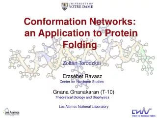
Center for Nonlinear Studies. Conformation Networks: an Application to Protein Folding. Zoltán Toroczkai. Erzsébet Ravasz. Center for Nonlinear Studies. Gnana Gnanakaran (T-10). Theoretical Biology and Biophysics. Los Alamos National Laboratory. Proteins.

E N D
Center for Nonlinear Studies Conformation Networks: an Application to Protein Folding Zoltán Toroczkai Erzsébet Ravasz Center for Nonlinear Studies Gnana Gnanakaran (T-10) Theoretical Biology and Biophysics Los Alamos National Laboratory
Proteins • the most complex molecules in nature • globular or fibrous • basic functional units of a cell • chains of amino acids (50 – 103) • peptide bonds link the backbone Native state • unique 3D structure (native physiological conditions) • biological function • fold in nanoseconds to minutes • about 1000 known 3D structures: X-ray crystallography, NMR
Myoglobin 153 Residues, Mol. Weight=17181 [D], 1260 Atoms Main function: primary oxygen storage and carrier in muscle tissue It contains a heme (iron-containing porphyrin ) group in the center. C34H32N4O4FeHO
Protein conformations Amino-acid • defined by dihedral angles • 2 angles with 2-3 local minima of the torsion energy • N monomers about 10N different conformations
Levinthal’s paradox • Anfinsen: thermodynamic hypothesis • native state is at the global minimum of the free energy Epstain, Goldberger, & Anfinsen, Cold Harbor Symp. Quant. Biol.28, 439 (1963) • Levinthal’s paradox, 1968 • finding the native state by random sampling is not possible • 40 monomer polypeptide 1013 conf/s 3 1019 years to sample all universe ~ 2 1010 years old Levinthal, J. Chim. Phys. 65, 44-45 (1968) Wetlaufer, P.N.A.S. 70, 691 (1973) • nucleation • folding pathways
Free energy landscapes • Bryngelson & Wolynes, 1987 • free energy landscape Bryngelson & Wolynes, P.N.A.S. 84, 7524 (1987) • a random hetero-polymer typically does NOT fold • Experiment: • random sequences • GLU, ARG, LEU • 80-100 amino-acids • ~ 95% did not fold • in a stable manner Davidson & Sauer, P.N.A.S.91, 2146 (1994)
Funnels Given any amino-acid sequence: can we tell if it is a good folder? • experiments (X-ray, NMR) • molecular dynamics simulations • homology modeling • Leopold, Mortal & Onuchic, 1992 Leopold, Mortal & Onuchic, P.N.A.S. 89, 8721 (1992) Energy funnels Difficult and slow • many folding pathways
Molecular dynamics Sanbonmatsu, Joseph & Tung, P.N.A.S. 102 15854 (2005) • State of the art • supercomputer (LANL) • Ribosome in explicit solvent: • targeted MD • 2.64x10⁶ atoms (2.5x10⁵ + water) • Q machine, 768 processors • 260 days of simulation (event: 2 ns) ~ 1016 times slower • distributed computing (Stanford, Folding@home) • more than 100,000 CPU’s • simulation of complete folding event • BBA5, 23-residue, implicit water • 10,000 CPU days/folding event (~1s) Shirts & Pande, Science290, 1903 (2000) Snow, Nguyen, Pande, Gruebele, Nature420,102 (2002)
Configuration networks Ramachandran map PDB structures • Configuration networks Protein conformations • dihedral angles have few preferred values Ramachandran & Sasisekharan, J.Mol.Biol.7, 95 (1963) • Helix • Sheet • other NODE configuration LINK change of one degree of freedom (angle) • refinement of angle values continuous case
Why networks? • VERY LARGE: 100 monomers 10100 nodes. However: Generic features of folding are determined by STATISTICAL properties of the configuration network • degree distribution • average distance • clustering • degree correlations • toolkit from network research • captures the high dimensionality Albert & Barabási, Rev. Mod. Phys.74, 67 (2002); Newman, SIAM Rev.45, 167 (2003) • faster algorithms to simulate folding events • pre-screening synthetic proteins • insights into misfolding
A real example • The Protein Folding Network: F. Rao, A. Caflisch, J.Mol.Biol, 342, 299 (2004) • beta3s: 20 monomers, antiparallel beta sheets • MD simulation, implicit water • 330K, equilibrium folded random coil NODE -- 8 letters / AA (local secondary struct) LINK -- 2ps transition
Its native conformation has been studied by NMR experiments: De Alba et.al. Prot.Sci. 8, 854 (1999). Beta3s in aqueous solution forms a monomeric triple-stranded antiparallel beta sheet in equilibrium with the denaturated state. • Simulations @ 330K • The average folding time from denaturated state ~ 83ns • The average unfolding time ~83ns • Simulation time ~12.6s • Coordinates saved at every 20ps (5105 snapshots in 10s) • Secondary structures: H,G,I,E,B,T,S,- (-helix, 310 helix, -helix, extended, isolated -bridge, hydrogen-bonded turn, bend and unstructured). • The native state: -EEEESSEEEEEESSEEEE- • There are approx. 818 1016 conformations. • Nodes: conformations, transitions: links.
Scale-free network Many real-world networks are scale free • hubs beta3s randomized • co-authorship (=1 - 2.5) • citations (=3) • sexual contacts (=3.4) • movie actors (=2.3) • Internet (y=2.4) • World Wide Web (=2.1/2.5) • Genetic regulation (=1.3) • Protein-protein interactions ( =2.4) • Metabolic pathways (=2.2) • Food webs (=1.1) Barabási & Albert, Science 286, 509, (1999); Many reasons behind SF topology • Why is the protein network scale free? • Why does the randomized chain have similar degree distribution? • Why is = - 2 ?
Robot arm networks 12 n=0 22 02 11 01 21 0 2 1 20 n=1 00 10 00 22 n=2 01 21 02 20 021 021 10 12 11 020 020 010 010 000 000 100 100 200 200 • Steric constraints? • missing nodes • missing links • n-dimensional hypercube • binomial degree distribution Homogeneous Swiss cheese
A bead-chain model • Beads on a chain in 3D: robot arm model • similar to C protein models • rod-rod angle • 3 positions around axis Honeycutt & Thirumalai, Biopolymers32, 695 (1992) N=6; = 90 N=18; = 120 2212112212111122 • Homogeneous network
Another example: L = 7, = 75 , r = 0.25 “00100” state “00100” allowed state forbidden state
Adding monomers not only increases the number of nodes in the network but also its dimensionality!! The combined effect is small-world.
The “dilemma” SCALE FREE • from polypeptide MD simulations • beta3s • randomized version HOMOGENEOUS • from studies of conformation networks • bead chain • robot arm ?
Gradient Networks Gradients of a scalar (temperature, concentration, potential, etc.) induce flows (heat, particles, currents, etc.). Naturally, gradients will induce flows on networks as well. Ex.: Load balancing in parallel computation and packet routing on the internet Y. Rabani, A. Sinclair and R. Wanka, Proc. 39th Symp. On Foundations of Computer Science (FOCS), 1998:“Local Divergence of Markov Chains and the Analysis of Iterative Load-balancing Schemes” References: Z. T. and K.E. Bassler, “Jamming is Limited in Scale-free Networks”, Nature, 428, 716 (2004) Z. T., B. Kozma, K.E. Bassler, N.W. Hengartner and G. Korniss “Gradient Networks”, http://www.arxiv.org/cond-mat/0408262
Setup: Let G=G(V,E) be an undirected graph, which we call the substrate network. The vertex set: The edge set: A simple representation of E is via the Nx N adjacency (or incidence) matrix A (1) Let us consider a scalar field Set of nearest neighbor nodes on G of i :
Definition 1 The gradient h(i) of the field {h} in node i is a directed edge: (2) Which points from i to that nearest neighbor for G for which the increase in the scalar is the largest, i.e.,: (3) The weight associated with edge (i,) is given by: . . The self-loop is a loop through i with zero weight. Definition 2 The set F of directed gradient edges on G together with the vertex set V forms the gradient network: If (3) admits more than one solution, than the gradient in i is degenerate.
In the following we will only consider scalar fields with non-degenerate gradients. This means: Theorem 1 Non-degenerate gradient networks form forests. Proof:
0.48 0.82 0.67 0.46 0.65 0.6 0.53 0.44 0.5 0.67 0.7 0.2 0.22 0.65 0.1 0.19 0.16 0.87 0.14 0.15 0.32 0.2 0.2 0.18 0.05 0.55 0.44 0.15 0.05 0.24 0.43 0.16 0.8 0.13 0.65 0.65 Theorem 2 The number of trees in this forest = number of local maxima of {h} on G.
For Erdős - Rényi random graph substrates with i.i.d random numbers as scalars, the in-degree distribution is:
The Configuration model A. Clauset, C. Moore, Z.T., E. Lopez, to be published.
Generating functions: K-th Power of a Ring
The energy landscape • Energy associated with each node (configuration) • the gradient network • most favorable transitions • T=0 backbone of the flow • MD simulation • tracks the flow network • biased walk close to the gradient network • trees • basins of local minima What generates = - 2 ? The REM generates an exponent of -1.
Model ingredients k, E increases constrained (folded) small kconf lower energy loose (random coil) large kconf higher energy • A network model of configuration spaces • network topology • homogeneous • degree correlations • how to associate energies
Random geometric graph R=0.113, <k>=20 • Energy proportional to connectivity E k • random geometric graph Dall & Christensen, Phys.Rev.E 66, 026121 (2002) • in higher D: similar to hypercube with holes • degree correlations
Exponent is - 2 2 essential ingredients: k1-k2 correlations <E> with k monotonic
Bead-chain model Lennard-Jones potential Repulsive Attractive • more realistic model: bead-chain • configuration network • excluded volume • energy: Lennard-Jones
The case of the -helix AKA peptide • ALA: orange • LYS: blue • TYR: green MD simulations, no water.
The MD traced network T = 400 More than one simulation 3 different runs: yellow, red and green The role of temperature
Conclusions • A network approach was introduced to study sterically constrained conformations of ball-chain like objects. • This networks approach is based on the “statistical dogma” stating that generic features must be the result of statistical properties of the networks and should not depend on details. • Protein conformation dynamics happens in high dimensional spaces that are not adequately described by simplistic reaction coordinates. • The dynamics performs a locally biased sampling of the full conformational network. For low enough temperatures the sampled network is a gradient graph which is typically a scale-free structure. • The -2 degree exponent appears at and bellow the temperature where the basins of the local energy minima become kinetically disconnected. • Understanding the protein folding network has the potential of leading to faster simulation algorithms towards closing the gap between nature’s speed and ours. Coming up: conditions on side chain distributions for the existence of funneled energy landscapes.