CH1. BASIC CONCEPTS
CH1. BASIC CONCEPTS. 1.1 System Life Cycle. Requirements Gathering : Types of expression Analysis Elimination of ambiguities, Partition of requirements Specification Define what the system is to do Functional specification Performance specification. 1.1 System Life Cycle(Cont ’ ).

CH1. BASIC CONCEPTS
E N D
Presentation Transcript
1.1 System Life Cycle • Requirements • Gathering : Types of expression • Analysis • Elimination of ambiguities, Partition of requirements • Specification • Define what the system is to do • Functional specification • Performance specification
1.1 System Life Cycle(Cont’) • Design • Description of how to achieve the specification • Data objects → Abstract data types • Operations → Algorithms • Programming language independent • Design approaches : Top-down / Bottom-up approach • Coding • Programming language dependent • Verification • Correctness proofs, Test, Error removal • Operation and maintenance • System installation, operation, System modification
1.2 Object-Oriented Design • Object-oriented design vs. structured programming design • similarity : divide and conquer • difference : decomposition method
1.2 Object-Oriented Design(Cont’) 1.2.1 Algorithmic Decomposition vs. Object-Oriented Decomposition • Algorithmic decomposition (Functional decomposition) • software = process • modules = steps of the process • Object-oriented decomposition • software = a set of objects that model entities and interact with each other • provides reusability, flexible to change
1.2 Object-Oriented Design(Cont’) 1.2.2 Fundamental Definitions and Concepts of Object-Oriented Programming • Object is an entity, performs computations • Object-oriented programming is a method of implementation • objects are the fundamental building blocks • each object is an instance of some type (class) • classes are related to each other by inheritance relationships • Object-oriented language : objects, class, inheritance
1.3 Data Abstraction and Encapsulation • Data encapsulation (Information hiding) • concealing of the implementation of a data object from the outside world • Data abstraction • separation of the specification of a data object from its implementation • C++ data types • fundamental data types • char, int, float, double • modifiers: short, long, signed, unsigned • derived data types • pointer, reference • grouping mechanisms • array, struct, class • user-defined data types
1.3 Data Abstraction and Encapsulation (Cont’) • Abstract Data Type(ADT) and Encapsulation objects (data) operations private public
1.3 Data Abstraction and Encapsulation (Cont’) ADT NaturalNumber is objects : An ordered subrange of integers starting at zero and ending at the maximum integer (MAXINT) on the computer. functions : for all x, y ∈ NaturalNumber, TRUE, FALSE ∈ Boolean +, -, <, ==, = are the usual integer operations Zero():NaturalNumber ::= 0 IsZero(x):Boolean ::= if (x == 0) IsZero = TRUE else IsZero = FALSE Add(x,y):NaturalNumber ::= if (x+y <= MAXINT) Add= x+y else Add = MAXINT Equal(x,y):Boolean ::= if (x == y) Equal = TRUE else Equal = FALSE end NaturalNumber ADT 1.1 : Abstract data type NaturalNumber
1.3 Data Abstraction and Encapsulation (Cont’) Figure 1.1 : Search area for bugs
1.3 Data Abstraction and Encapsulation (Cont’) • Advantages of data abstraction and encapsulation • simplification of software development • decomposition of complex task into simpler tasks • efficient testing and debugging • amount of code to be searched • enhance the reusability • easy modifications to the representations of a data type • implementation of a data type is not visible to the rest of the program • change of a part of the shaded area
1.3 Data Abstraction and Encapsulation (Cont’) rest of the program operation implementation of operations internal representation of data type Data type
1.4 Basics of C++ 1.4.1 Program Organization in C++ • Header file • .h suffix • store declarations • system-defined (iostream.h) or user-defined • #include preprocessor directive is used • Source file • .c suffix • store C++ source code
1.4 Basics of C++(Cont’) 1.4.2 Scope in C++ • File scope • to access a global variable locally • use the scope operator :: • to use in file2.c a global variable defined in file1.c • use extern to declare a variable in file2.c • both file1.c and file2.c define the same global variable for different entities • use static to declare in both files • Function scope • Local scope • Class scope
1.4 Basics of C++(Cont’) 1.4.3 C++ Statements and Operators • C++ operators : identical to C operators • Exceptions • new and delete for dynamic memory management • >> and << for input and output • operator overloading
1.4 Basics of C++(Cont’) 1.4.4 Data Declarations in C++ • same as C declarations except the reference type (1) Constant values (2) Variables (3) Constant variables (4) Enumeration types • example : enum Boolean {FALSE, TRUE}; (5) Pointers • hold memory address of objects • example : int i=25; int *np; np=&i; (6) Reference types • an alternate name for an object • example : int i=5; int& j=i; i=7; printf("i=%d, j=%d", i, j);
1.4 Basics of C++(Cont’) 1.4.6 Input/Output in C++ #include <iostream.h> main() { int a,b; cin>>a>>b; } #include <iostream.h> main() { int n=50; float f=20.3; cout<<"n:"<<n<<endl; cout<<"f:"<<f<<endl; } Program 1.1: Output in C++ Program 1.2 : Input in C++ Input 1 5 10 <Enter> Input 2 5 <Enter> 10 <Enter> Output n : 50 f : 20.3
1.4 Basics of C++(Cont’) • Advantages of I/O in C++ • format-free : no formatting symbols • I/O operators can be overloaded • File I/O in C++ • include the header file fstream.h
1.4 Basics of C++(Cont’) 1.4.6 Input/Output in C++(Con’t) #include <iostream.h> #include <fstream.h> main() { ofstream outFile("my.out", ios::out); if (!outFile) { cerr<<"cannot open my.out"<<endl;//standard error device return; } int n = 50; float f = 20.3; outFile << "n: " << n << endl; outFile << "f: " << f << endl; } Program 1.3 : File I/O in C++
1.4 Basics of C++(Cont’) 1.4.7 Functions in C++ • regular functions • member functions of specific C++ classes
1.4 Basics of C++(Cont’) 1.4.8 Parameter Passing in C++ • Pass by value : object is copied • Pass by reference : address of object is copied • Pass by constant reference • retain the advantages of both methods • const T& a • Array types • default is pass by reference • a point to the first element of an array is passed
1.4 Basics of C++(Cont’) 1.4.9 Function Name Overloading in C++ • More than one function with the same name int max(int, int) ; int max(int, int, int) ; int max(int*, int) ;
1.4 Basics of C++(Cont’) 1.4.10 Inline Functions inline int sum(int a, int b) { return a+b ; } • i=sum(x, 12) is replaced by i=x+12
1.4 Basics of C++(Cont’) 1.4.11 Dynamic Memory Allocation in C++ • Allocation/release to free store during runtime • new operator • creates an object of the desired type • returns a pointer to data type that follows new • if unable to create, the object, returns 0 • delete operator • an object created by new is deleted • delete is applied to a pointer to the object • example int *ip = new int; if (ip == 0) cerr << "Memory not allocated" << endl; ….. delete ip;
1.5 Algorithm Specification 1.5.1 Introduction • Algorithm • a finite set of instructions, if followed, accomplishes a particular task • Criteria • input ≥ 0 • output ≥ 1 • definiteness • finiteness • effectiveness : feasible • Program • does not have to satisfy finiteness • used interchangeably
1.5 Algorithm Specification(Cont’) • Description of an algorithm • a natural language like English • pseudo code • programming language : C++ • combination
1.5 Algorithm Specification(Cont’) • Example [Selection sort] • a program that sorts a collection of n≥1 integers • from those integers that are currently unsorted, find the smallest and place it next in the sorted list for (int i = 0; i < n; i++) { examine a[i] to a[n-1] and suppose the smallest integer is at a[j]; interchange a[i] and a[j]; } Program 1.5 : Selection sort algorithm
1.5 Algorithm Specification(Cont’) void sort(int *a, const int n) // sort the n integers a[0] to a[n-1] into nondecreasing order { for (int i = 0; i < n; i++) { int j = i; // find smallest integer in a[i] to a[n-1] for (int k = i + 1; k < n; k++) if (a[k] < a[j]) j = k; // interchange int temp = a[i]; a[i] = a[j]; a[j] = temp; } } Program 1.6 : Selection sort
1.5 Algorithm Specification(Cont’) a[0] a[1] a[2] a[3] 5 4 13 2 i=0 2 4 13 5 i=1 2 4 13 5 i=2 2 4 5 13
1.5 Algorithm Specification(Cont’) • Theorem • sort(a, n) correctly sorts a set of n≥1 integers • Proof • for any i, say i=q, after steps 6-11, a[q]≤a[r] for q<r≤n-1 • when i>q, a[0]...a[q] is unchanged • when i=n-1, a[0]≤a[1]≤...≤a[n-1]
1.5 Algorithm Specification(Cont’) • Example [Binary search] • n≥1 distinct integers are already sorted in the array a[0]...a[n-1] • if the integer x is present, return j such that x=a[j] otherwise return • left, right : the left and right ends of the list to be searched(initially:0, n-1) • middle = (left + right)/2 • compare a[middle] with x (1) x<a[middle] : right = middle-1 (2) x=a[middle] : return middle (3) x>a[middle] : left = middle+1 • two subtasks (1) determine if there are any integers left to check (2) compare x to a[middle]
1.5 Algorithm Specification(Cont’) char compare(int x, int y) { if (x > y) return '>'; else if (x < y) return '<'; else return '='; } // end of compare } Program 1.7 : Comparing two elements
1.5 Algorithm Specification(Cont’) int BinarySearch(int *a, const int x, const int n) // Search the sorted array a[0], ..., a[n-1] for x { for (int left = 0, right = n-1; left <= right;) { // while more elements int middle = (left + right) / 2; switch (comare(x,a[middle])) { case '>' : left = middle + 1; break; // x > a[middle] case '<' : right = middle - 1; break; // x < a[middle] case '=' : return middle; // x == a[middle] } // end of switch } // end of for return -1; // not found } // end of BinarySearch Program 1.9 : C++ function for binary search
1.5 Algorithm Specification(Cont’) 1.5.2 Recursive Algorithms • Example [Factorial] • N! = N*(N-1)! int Fact (int N) { if N=0 return (1); else return (N*Fact(N-1)); }
1.5 Algorithm Specification(Cont’) • Example [Recursive binary search] int BinarySearch(int *a, const int x, const int left, const int right) // Search the sorted array a[left], ..., a[right] for x { if(left <= right) { int middle = (left + right) / 2; switch(compare(x, a[middle])) { case '>' : return BinarySearch(a, x, middle+1, right); // x > a[middle] case '<' : return BinarySearch(a, x, left, middle-1); // x < a[middle] case '=' : return middle; // x == a[middle] } // end of switch } // end of if return -1; // not found } // end of BinarySearch Program 1.10 : Recursive implementation of binary search
1.6 Performance Analysis and Measurement • Program complexity • space complexity : the amount of memory it needs • time complexity : the amount of computer time it needs • Performance evaluation phases • performance analysis : a priori estimates • performance measurement : a posteriori testing
1.6 Performance Analysis and Measurement(Cont’) 1.6.1 Performance Analysis • Space complexity • fixed part : independent of the characteristics of the inputs and outputs • variable part : depends on the instance characteristics • S(P) = c+Sp(instance characteristics) • S(P):space requirement of program P • c : constant • Example [Iterative sum] • the problem instances are characterized by n • n is passed by value : 1 word is allocated • a is the address of a[0], 1 word is needed • the space is independent of n: Sp(n)=0
1.6 Performance Analysis and Measurement(Cont’) line float sum(float *a, const int n) 1 { 2 float s = 0; 3 for(int i = 0; i < n; i++) 4 s += a[i]; 5 return s; 6 } Program 1.13 : Iterative function for sum
1.6 Performance Analysis and Measurement(Cont’) • Example [Recursive sum] • the problem instances are characterized by n • the depth of recursion depends on n : it is n+1 • each call requires at least 4 words : n, a, returned value, return address • the recursion stack space is 4(n+1)
1.6 Performance Analysis and Measurement(Cont’) line float rsum(float *a, const int n) 1 { 2 if(n <= 0) return 0; 3 else return (rsum(a, n-1)+a[n-1]); 4 } Program 1.14 : Recursive function for sum
1.6 Performance Analysis and Measurement(Cont’) • Time complexity T(P) = c + Tp(n) • T(P) : time taken by program P • c : compile time • Tp : run time • n : instance characteristics • Program step • a meaningful segment of a program • execution time is independent of the instance characteristics • the number of steps of a program statement : depends on the nature of the statement • determine the number of steps of a program • introduce a new variable, count, into the program • build a table to list steps by each statement
1.6 Performance Analysis and Measurement(Cont’) • Example of count [Iterative sum] line float sum(float *a, const int n) 1 { 2 float s = 0; 3 for(int i = 0; i < n; i++) 4 s += a[i]; 5 return s; 6 } line float rsum(float *a, const int n) 1 { 2 if(n <= 0) return 0; 3 else return (rsum(a, n-1)+a[n-1]); 4 } Program 1.13 : Iterative function for sum Program 1.14 : Recursive function for sum
1.6 Performance Analysis and Measurement(Cont’) Example [Recursive sum] Example [Iterative sum] line s/e frequency total steps Line s/e* frequency total steps 1 0 1 0 n=0 n>0 n=0 n>0 2 1 1 1 1 0 1 1 0 0 3 1 n+1 n+1 2(a) 1 1 1 1 1 4 1 n n 2(b) 1 1 0 1 0 5 1 1 1 3 1+trsum(n-1) 0 1 0 1+trsum(n-1) 6 0 1 0 4 0 1 1 0 0 Total number of steps 2n+3 Total number of steps 2 2+trsum(n-1) Table 1.1 Step table for Program 1.13 Table 1.2 Step table for Program 1.14 (*s/e : step per execution)
1.6 Performance Analysis and Measurement(Cont’) • Solution of recurrence relation trsum(n) = 2 + trsum(n-1) = 2 + 2 + trsum(n-2) = 2 * 2 + trsum(n-2) …… = 2n + trsum(0) = 2n + 2
1.6 Performance Analysis and Measurement(Cont’) • Three kinds of step counts • best-case • worst-case • average
1.6 Performance Analysis and Measurement(Cont’) • Asymptotic notation (O, Ω, Θ) • determining the exact step count is very difficult • the notion of a step is inexact • Definition [Big "oh"] • f(n)=O(g(n)) iff there exist positive constants c and n0 such that f(n)≤cg(n) for all n, n≥n0 • 3n+3= O(n) as 3n+3≤4n for all n≥3 • 3n+3=O(n2) as 3n+3≤3n2 for n≥2 • g(n) is an upper bound
1.6 Performance Analysis and Measurement(Cont’) • Definition [Omega] • f(n)=Ω(g(n)) iff there exist positive constants c and n0 such that f(n)≥cg(n) for all n, n≥n0 • g(n) is a lower bound ex) 3n+2=Ω(n) • 10n2+4n+2=Ω(n2) • Definition [Theta] • f(n)=Θ(g(n)) iff there exist positive constants c1, c2 and n0 such that c1g(n)≤f(n)≤c2g(n) for all n, n≥n0 • g(n) is both an upper and lower bound ex) 3n+2=Θ(n) 10n2+4n+2=Θ(n2) 6×2n+n2=Θ(2n)
1.6 Performance Analysis and Measurement(Cont’) • Asymptotic complexity(in terms of O,Ω,Θ) • easily determined without determining the exact step count line (s) s/e frequency total steps 1 0 - (0) 2 1 1 (1) 3 1 n+1 (n) 4 1 n (n) 5 1 1 (1) 6 0 - (0) Tsum(n)=Θ(max {gi(n)}) = Θ(n), 1≤i≤6 Table1.4:Asymptotic Complexity of sum (Program 1.13)
1.6 Performance Analysis and Measurement(Cont’) • Practical complexities • for large n, only programs of small complexity are feasible Figure 1.3 : plot of function values