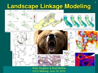
Landscape Linkage Modeling
1. Landscape Linkage Modeling. Prepared by Peter Singleton, USFS PNW Research Station for the State-wide CCLC Meeting, July 28, 2008. 2. Introduction. Definitions of connectivity:
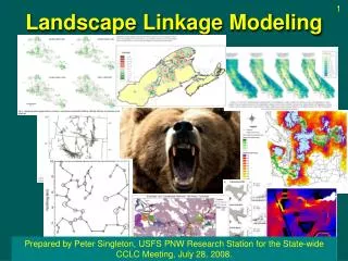

Landscape Linkage Modeling
E N D
Presentation Transcript
1 Landscape Linkage Modeling Prepared by Peter Singleton, USFS PNW Research Station for the State-wide CCLC Meeting, July 28, 2008.
2 Introduction Definitions of connectivity: Merriam 1984: The degree to which absolute isolation is prevented by landscape elements which allow organisms to move among patches. Taylor et al 1993: The degree to which the landscape impedes or facilitates movement among resource patches. With et al 1997: The functional relationship among habitat patches owing to the spatial contagion of habitat and the movement responses of organisms to landscape structure. Singleton et al 2002: The quality of a heterogeneous land area to provide for passage of animals (landscape permeability).
3 Introduction • Structural Connectivity: The spatial arrangement of different types of habitat or other elements in the landscape. • Functional Connectivity: The behavioral response of individuals, species, or ecological processes to the physical structure of the landscape. • Potential Connectivity • Actual Connectivity
4 Introduction Darwin’s Finches - 1837: Images from Robert Rothman http://people.rit.edu/rhrsbi/GalapagosPages/DarwinFinch.html
5 Introduction Island Biography • MacArthur & Wilson 1967 The Theory of Island Biogeography Reserve Design • Soule 1987 Viable Populations for Conservation • Meffe & Carroll 1994 Conservation Biology Textbook Conservation Corridors • Servheen & Sandstrom 1993 Linkage Zones for Grizzly Bears… End. Sp. Bul. 18 • Walker & Craighead 1997 Analyzing Wildlife Movement Corridors… Proc. ESRI Users Conf. • Around 2000, linkage assessment workshops start happening • Mid-2000’s, lots of publications addressing corridors / connectivity Landscape Processes • Late-2000’s Maturation of landscape genetics • Future? More empirical data relating landscape process and pattern?
6 Introduction From: Crooks & Sanjayan. 2006. Connectivity Conservation. Cambridge Univ. Press
7 Analysis Approaches • Patch Metrics • Graph Theory • Cost-distance Analysis • Combining graph theory and cost-distance • Circuit Theory • Individual-based & Population Viability Models • Patch / HexSim
8 Analysis Approaches Simple Few Assumptions Needs Less Input Info Structural focus • Patch Metrics • Graph Theory • Cost-distance Analysis • Combining graph theory and cost-distance • Circuit Theory • Individual-based & Population Viability Models • Patch / HexSim Complex Lots of Assumptions Needs More Input Info Process focus
9 Analysis Approaches 1) Patch Metrics • Quantifies Patch Characteristics or Relationships Between Patches (e.g. patch size, nearest neighbor) • Emphasizes Structural Connectivity • Generally must be summarized across a landscape unit (e.g. watershed or planning unit) • Very useful for quantifying landscape patterns (e.g. historic range of variability, monitoring change, comparing landscapes) • Structure, not process oriented • Don’t provide a lot of information about expected movement patterns
10 Landscape Metric Example – Effective Mesh Size From: Girvetz, Thorne, & Jaeger. 2007. Integrating Habitat Fragmentation Analysis into Transportation Planning Using The Effective Mesh Size Landscape Metric. 2007 ICOET Proceedings.
Landscape Metric Example – Effective Mesh Size 11 From: Girvetz, Thorne, & Jaeger. 2007. Integrating Habitat Fragmentation Analysis into Transportation Planning Using The Effective Mesh Size Landscape Metric. 2007 ICOET Proceedings.
12 Analysis Approaches 2) Graph Theory • Focused on quantifying relationships between patches • More focused on process • Solidly based in mathematical theory with many applications in other fields (e.g. geography, computer science, logistics) • Provides a language for describing relationships between patches
13 Graph Theory • Vocabulary: • Patch (Node) – the points of interest • Link (Edge) – connections between the nodes • Path – a sequence of connected nodes • Tree – a set of paths that do not return to the same node • Spanning Tree – a tree that includes every node in the graph • Connected Graph – a graph with a path between every pair of nodes • Component (Subgraph) – part of the graph where every node is adjacent to another node in that part of the graph • Node-connectivity – the minimum number of nodes that must be removed from a connected graph before it becomes disconnected • Line-connectivity – the minimum number of links that must be removed before a graph becomes disconnected From: Urban & Keitt. 2001. Landscape Connectivity: A graph-theoretic approach. Ecology 82:1205-1218
14 Graph Theory From: Urban & Keitt. 2001. Landscape Connectivity: A graph-theoretic approach. Ecology 82:1205-1218
15 Graph Theory From: Urban & Keitt. 2001. Landscape Connectivity: A graph-theoretic approach. Ecology 82:1205-1218
16 Analysis Approaches 3) Cost-distance Analysis • More focus on matrix • Can quantify isolation between patches • Spatially explicit – can identify routes and bottlenecks • Based on the concept of “movement cost” that has some foundation in ecological theory, but lacks extensive empirical documentation • Several important assumptions about parameters and scale must be considered
Cost-distance Analysis 17 Habitat Suitability: 0 = Barrier 1 = Poor 2 = Moderate 3 = Good 10 = Source Analysis Steps: • Identify Patches • Develop Friction Surface • Evaluate Landscape Travel Cost: 0 = 99 1 = 3 2 = 2 3 = 1 10 = Source Cost-distance 22 16 There are critical assumptions at each one of these steps!
Cost-distance Analysis 18 Results from cost-distance analysis: • Minimum cost-distance • Cost / Euclidean ratios • nth best corridor area delineations • Spatially explicit maps Many cost-distance applications have failed to take advantage of this information by focusing on least-cost paths or corridors (“Failing to see the landscape for the corridor”)
Cost-distance Analysis 19 Step 1: Identifying source patches: Large roadless areas and units highlighted in focal species management plans. From: Singleton et al. 2002. Landscape Permeability for Large Carnivores in Washington: A Weighted-Distance and Least-Cost Corridor Assessment. USFS PNW Research Station PNW-RP-549
Cost-distance Analysis 20 Step 2: Develop friction surface • Cost Model Parameters: • Population Density • 0 - 10 people/mi2 1.0 • 10 - 25 people/mi2 0.8 • 25 - 50 people/mi2 0.5 • 50 - 100 people/mi2 0.3 • >100 people/mi2 0.1 • Road Density • < 1mi/mi2 1.0 • 1 - 2 mi/mi2 0.8 • 2 - 6 mi/mi2 0.5 • 6 - 10 mi/mi2 0.2 • >10 mi/mi2 0.1 • Land Cover • All Forest & Wetlands 1.0 • Alpine, shrub, 0.8 • grasslands • Agriculture, bare 0.3 • Water, urban, ice 0.1 • Slope • 0 - 20% 1.0 • 20 - 40% 0.8 • >40% 0.6 Road Density Land Cover From: Singleton et al. 2002. Landscape Permeability for Large Carnivores in Washington: A Weighted-Distance and Least-Cost Corridor Assessment. USFS PNW Research Station PNW-RP-549
21 Cost-distance Analysis Step 2: Develop friction surface From: Singleton et al. 2002. Landscape Permeability for Large Carnivores in Washington: A Weighted-Distance and Least-Cost Corridor Assessment. USFS PNW Research Station PNW-RP-549
22 Cost-distance Analysis Step 2: Develop friction surface From: Singleton et al. 2002. Landscape Permeability for Large Carnivores in Washington: A Weighted-Distance and Least-Cost Corridor Assessment. USFS PNW Research Station PNW-RP-549
Cost-distance Analysis 23 Step 3: Evaluate the landscape From: Singleton et al. 2002. Landscape Permeability for Large Carnivores in Washington: A Weighted-Distance and Least-Cost Corridor Assessment. USFS PNW Research Station PNW-RP-549
Cost-distance Analysis 24 Step 3: Evaluate the landscape From: Singleton et al. 2002. Landscape Permeability for Large Carnivores in Washington: A Weighted-Distance and Least-Cost Corridor Assessment. USFS PNW Research Station PNW-RP-549
Fracture Zone Minimum Cost Distance (km) Actual Linear Distance (km) Cost Distance / Linear Distance Ratio Fraser River Canyon 288.1 27.9 10.3 Upper Columbia River 423.5 46.3 9.1 I-90 Snoqualmie Pass 630.4 33.5 18.8 Okanogan Valley 633.5 80.8 7.8 Southwestern Washington 6943.8 116.2 82.6 Cost-distance Analysis 25 Step 3: Evaluate the landscape Pretty easy to understand with a simple patch – linkage structure, but when things get more complex… From: Singleton et al. 2002. Landscape Permeability for Large Carnivores in Washington: A Weighted-Distance and Least-Cost Corridor Assessment. USFS PNW Research Station PNW-RP-549
26 A Digression: Integrating Cost-Distance Analysis and Graph Theory From: O’Brien et al 2006. Testing the importance of spatial configuration of winter habitat for woodland Caribou: an application of graph theory. Biological Conservation 130:70-83.
27 A Digression: Integrating Cost-Distance Analysis and Graph Theory FunConn ArcGIS Toolbox: http://www.nrel.colostate.edu/projects/starmap/ From: Theobald et al. 2006. FunConn v1 User’s Manual: ArcGIS tools for Functional Connectivity Modeling. Colorado State University.
28 Analysis Approaches 4) Circuit Theory • Based on electrical engineering theory • Generates a measure of “flow” through each cell in a landscape • Integrates all possible pathways into calculations • Corresponds well with random-walk models • Resistance measures can be used in graph-theory applications From: McRae et al. in press. Using Circuit Theory to Model Connectivity in Ecology, Evolution, and Conservation. Ecology (expected publication fall 2008).
Simple landscapes Resistance distance Least-cost path distance 29 A B C D E F Slide by Brad McRae
High Low 30 A more realistic landscape Circuit theory: Least-cost path: Slide by Brad McRae
Analysis Approaches 31 5) Individual Based Models & Other Approaches • Individual-based movement models (IBM) • Simulates movement of an individual through the landscape (e.g. PATH) • Many scales, from dispersal (coarse) to foraging (fine) • Population viability models (PVA) • Uses demographic information to project population persistence (e.g. Vortex) • Spatially explicit population models (SEPMs) • Integrates PVA with a heterogeneous landscape where vital rates vary (e.g. Ramas GIS)
32 • HexSim (updated version of Patch): • IBM & SEPM • Each cell represents a female home range • Survival / reproduction / dispersal probabilities are related to the habitat characteristics of the cell • Models individual dispersal movements through the landscape • Assumes territorial, non-social behavior (originally developed for spotted owl PVA) • Developed by Nathan Schumacher, EPA, Corvallis OR (http://www.epa.gov/hexsim/) Individual-based model example: Patch / HexSim
Individual-based model example: Patch / HexSim 33 From: USFWS 2008. Final Recovery Plan for the Northern Spotted Owl. May 2008. USFWS Region 1, Portland OR. Analysis by Marcot & Raphael Images by Bruce Marcot
Individual-based model example: Patch / HexSim 34 From: Carroll 2005. Carnivore Restoration in the Northeastern U.S. and Southeastern Canada: A Regional-Scale Analysis of Habitat and Population Viability for Wolf, Lynx, and Marten. Wildlands Project – Special Paper No. 2. Richmond VA
35 Discussion Different approaches provide different information and require different inputs and assumptions Information Data Model Provided Inputs Assumptions Focus Landscape Metrics Less Less Fewer (implicit) Structure Graphs Cost-distance Circuit Theory IBM / SEPM More More More (explicit) Function
36 Discussion All of these modeling approaches involve major assumptions about: • Habitat associations • Parameterizing source areas or habitat patch characteristics • Dispersal behavior • Resistance to movement Some projects have addressed some of these issues by using parameters based on empirical RSFs, but assumptions about dispersal habitat selection remain difficult.
37 Discussion The future of linkage modeling • Better empirical techniques: • Integration of detection probability and movement probabilty into resource selection analysis • Model validation: • Landscape genetics • GPS telemetry studies
38 Closing Pete’s cornball philosophy of landscape modeling: • Know your question • Know your data • Keep it simple • Own your assumptions • Be open to surprises, but always check twice • All models are wrong, but some models are useful • Validate, validate, validate …