Chi-Square and F Distributions
530 likes | 881 Vues
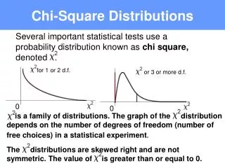
Chapter 11. Chi-Square and F Distributions. Understandable Statistics Ninth Edition By Brase and Brase Prepared by Yixun Shi Bloomsburg University of Pennsylvania. The Chi-Square Distribution. The χ 2 distribution has the following features: All possible values are positive.

Chi-Square and F Distributions
E N D
Presentation Transcript
Chapter 11 Chi-Square and F Distributions Understandable Statistics Ninth Edition By Brase and Brase Prepared by Yixun Shi Bloomsburg University of Pennsylvania
The Chi-Square Distribution • The χ2 distribution has the following features: • All possible values are positive. • The distribution is determined solely by the degrees of freedom. • The graph of the distribution is skewed right, but as the degrees of freedom increase, the distribution becomes more bell-shaped. • The mode of the distribution is at n – 2 (for sample sizes greater than 3).
Table 7 in Appendix II • The table gives critical values for area that falls to the right of the critical value.
Chi-Square: Test of Independence • The goal of the test is to determine if one qualitative variable is independent of another qualitative variable. • The hypotheses of the test: H0: The variables are independent H1: The variables are not independent
Chi-Square: Test of Independence • The data will be presented in a contingency table in which the rows will represent one variable and the columns will represent the other variable.
Chi-Square: Test of Independence • First, we need to compute the expected frequency, E, in each cell.
Chi-Square: Test of Independence • The sample statistic for the test will be: O = the observed frequency in each cell E = the expected frequency in each cell n = the total sample size
Chi-Square: Test of Independence • To use Table 7 to estimate the P-value of the test, the degrees of freedom are:
Test of Homogeneity • A test of homogeneity tests the claim that different populations share the same proportions of specified characteristics. • Test of homogeneity is also conducted using contingency tables and the chi-square distribution.
Test of Homogeneity Obtain random samples from each of the population. For each population, determine the numbers that share a distinct specified characteristic. Make a contingency table with the different populations as the rows (or columns) and the characteristics as the columns (or rows). The values recorded in the cells of the table are the observed value O taken from the samples. • Set the level of significance and use the hypotheses H0: The proportion of each population sharing specified characteristics is the same for all populations. H1: The proportion of each population sharing specified characteristics is not the same for all populations. 2. Follow steps 2—5 of the procedure used to test for independence.
Chi-Square: Goodness of Fit • We will test whether a given data set “fits” a given distribution. H0: The population fits the given distribution. H1: The population has a different distribution.
Testing σ2 • If we have a normal population with variance σ2and a random sample of n measurements with sample variance s2, then has a chi-square distribution with n – 1 degrees of freedom.
Working with theChi-Square Distribution Use Table 7 in Appendix II.
Confidence Intervals for σ2 Confidence Intervals for σ
Testing Two Variances • Assumptions: • The two populations are independent of each other. • Both populations have a normal distribution (not necessarily the same).
Notation • We choose population 1 to have the larger sample variance, i.e. s21 ≥ s22.
Compute the Test Statistic We will compare the test statistic to an F distribution, found in Table 8 of Appendix II.
Testing Two VariancesUsing F Distribution • Use the F-distribution and the type of test tofind or estimate the P-value with Table 8 of Appendix II. • Conclude the test. If P-value , then rejectH0. Otherwise do not reject H0. • Interpret your conclusion in the context of the application.
Using Table 8 Estimate the P-Value for F = 55.2 with d.f.N = 3 and d.f.D = 2
One-Way ANOVA • ANOVA is a method of comparing the means of multiple populations at once instead of completing a series of 2-population tests.
Establishing the Hypotheses in ANOVA In ANOVA, there are k groups and k group means. The general problem is to determine if there exists a difference among the group means.
Two-Way ANOVA • Two-Way ANOVA is a statistical technique to study two variables simultaneously. • Each variable is called a factor. • Each factor can have multiple levels. • We can study the different means of the factors as well as the interaction between the factors.
Steps For Two-Way ANOVA • Establish the hypotheses. • Compute the Sums of Squares Values. • Compute the Mean Squares Values. • Compute the F Statistic for each factor and the interaction. • Conclude the test.