Download

1 / 13
140 likes | 387 Vues
Chapter 10. Chi-Square Tests and the F - Distribution. Independence. § 10.2. Age. Gender. 16 – 20. 21 – 30. 31 – 40. 41 – 50. 51 – 60. 61 and older. Male. 32. 51. 52. 43. 28. 10. Female. 13. 22. 33. 21. 10. 6. Contingency Tables.

E N D
Chapter 10 Chi-Square Tests and the F-Distribution
Independence § 10.2
Age • Gender • 16 – 20 • 21 – 30 • 31 – 40 • 41 – 50 • 51 – 60 • 61 and older • Male • 32 • 51 • 52 • 43 • 28 • 10 • Female • 13 • 22 • 33 • 21 • 10 • 6 Contingency Tables An r c contingency table shows the observed frequencies for two variables. The observed frequencies are arranged in r rows and c columns. The intersection of a row and a column is called a cell. The following contingency table shows a random sample of 321 fatally injured passenger vehicle drivers by age and gender. (Adapted from Insurance Institute for Highway Safety)
Expected Frequency Assuming the two variables are independent, you can use the contingency table to find the expected frequency for each cell. Finding the Expected Frequency for Contingency Table Cells The expected frequency for a cell Er,cin a contingency table is
Age • Gender • 16 – 20 • 21 – 30 • 31 – 40 • 41 – 50 • 51 – 60 • 61 and older • Total • Male • 32 • 51 • 52 • 43 • 28 • 10 • 216 • Female • 13 • 22 • 33 • 21 • 10 • 6 • 105 • Total • 45 • 73 • 85 • 64 • 38 • 16 • 321 Expected Frequency Example: Find the expected frequency for each “Male” cell in the contingency table for the sample of 321 fatally injured drivers. Assume that the variables, age and gender, are independent. Continued.
Age • Gender • 16 – 20 • 21 – 30 • 31 – 40 • 41 – 50 • 51 – 60 • 61 and older • Total • Male • 32 • 51 • 52 • 43 • 28 • 10 • 216 • Female • 13 • 22 • 33 • 21 • 10 • 6 • 105 • Total • 45 • 73 • 85 • 64 • 38 • 16 • 321 Expected Frequency Example continued:
Chi-Square Independence Test A chi-square independence test is used to test the independence of two variables. Using a chi-square test, you can determine whether the occurrence of one variable affects the probability of the occurrence of the other variable. For the chi-square independence test to be used, the following must be true. • The observed frequencies must be obtained by using a random sample. • Each expected frequency must be greater than or equal to 5.
Chi-Square Independence Test The Chi-Square IndependenceTest If the conditions listed are satisfied, then the sampling distribution for the chi-square independence test is approximated by a chi-square distribution with (r – 1)(c – 1) degrees of freedom, where r and c are the number of rows and columns, respectively, of a contingency table. The test statistic for the chi-square independence test is where O represents the observed frequencies and E represents the expected frequencies. The test is always a right-tailed test.
Chi-Square Independence Test Performing a Chi-Square Independence Test In Words In Symbols • Identify the claim. State the null and alternative hypotheses. • Specify the level of significance. • Identify the degrees of freedom. • Determine the critical value. • Determine the rejection region. State H0 and Ha. Identify . d.f. = (r – 1)(c – 1) Use Table 6 in Appendix B. Continued.
Chi-Square Independence Test Performing a Chi-Square Independence Test In Words In Symbols • Calculate the test statistic. • Make a decision to reject or fail to reject the null hypothesis. • Interpret the decision in the context of the original claim. If χ2 is in the rejection region, reject H0. Otherwise, fail to reject H0.
Age • Gender • 16 – 20 • 21 – 30 • 31 – 40 • 41 – 50 • 51 – 60 • 61 and older • Total • Male • 32 (30.28) • 51 (49.12) • 52 (57.20) • 43 (43.07) • 28 (25.57) • 10 (10.77) • 216 • Female • 13 (14.72) • 22 (23.88) • 33 (27.80) • 21 (20.93) • 10 (12.43) • 6 (5.23) • 105 • 45 • 73 • 85 • 64 • 38 • 16 • 321 Chi-Square Independence Test Example: The following contingency table shows a random sample of 321 fatally injured passenger vehicle drivers by age and gender. The expected frequencies are displayed in parentheses. At = 0.05, can you conclude that the drivers’ ages are related to gender in such accidents?
Chi-Square Independence Test Example continued: Because each expected frequency is at least 5 and the drivers were randomly selected, the chi-square independence test can be used to test whether the variables are independent. H0: The drivers’ ages are independent of gender. Ha:The drivers’ ages are dependent on gender. (Claim) d.f. = (r – 1)(c – 1) = (2 – 1)(6 – 1) = (1)(5) = 5 With d.f. = 5 and = 0.05, the critical value is χ20 = 11.071. Continued.
O • E • O – E • (O – E)2 Rejection region • 32 • 30.28 • 1.72 • 2.9584 • 0.0977 • 51 • 49.12 • 1.88 • 3.5344 • 0.072 • 52 • 57.20 • 5.2 • 27.04 • 0.4727 • 43 • 43.07 • 0.07 • 0.0049 • 0.0001 • 28 • 25.57 • 2.43 • 5.9049 • 0.2309 X2 χ20 = 11.071 • 10 • 10.77 • 0.77 • 0.5929 • 0.0551 • 13 • 14.72 • 1.72 • 2.9584 • 0.201 • 22 • 23.88 • 1.88 • 3.5344 • 0.148 • 33 • 27.80 • 5.2 • 27.04 • 0.9727 • 21 • 20.93 • 0.07 • 0.0049 • 0.0002 • 10 • 12.43 • 2.43 • 5.9049 • 0.4751 • 6 • 5.23 • 0.77 • 0.5929 • 0.1134 Chi-Square Independence Test Example continued: Fail to reject H0. There is not enough evidence at the 5% level to conclude that age is dependent on gender in such accidents.