Download
1 / 23
260 likes | 512 Vues
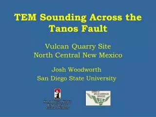
Audio Magnetotelluric Analysis of the Tanos Fault Area. SAGE 2007 Espa ñola Basin, NM. Overview. Area of Study Introduction to Magnetotellurics Data Acquisition 2-D Modeling Analysis Conclusions. Area of Study. Vulcan Quarry Site, Sandoval County, NM. Proposed Tanos Fault.

E N D
Audio Magnetotelluric Analysis of the Tanos Fault Area SAGE 2007 Española Basin, NM
Overview • Area of Study • Introduction to Magnetotellurics • Data Acquisition • 2-D Modeling • Analysis • Conclusions
Area of Study • Vulcan Quarry Site, Sandoval County, NM Proposed Tanos Fault
Magnetotellurics • The MT method uses natural variations in the magnetosphere to probe deep into the earth. • There are two main sources of these variations: • Lightning: Higher Frequency Variations • Solar Phenomena: Lower Frequency Variations
Data Aquisition • To supplement natural field variations, a Stratagem 400 A-m2 transmitter was used to boost field strength in the 1-50 kHz range. • We acquired data from 10 Hz- 100 kHz
Data Aquisition • Data was obtained at 6 stations. • Station spacing was 100m. • Station line was centered across the Tanos fault. • In each data set noise was masked manually. • Data was rotated through 30 degrees. • No other data editing techniques were used.
2-D Inversion Models • Many different models were run • Smoothness of models are governed by equation: • = d +m • d = misfit • m = roughness • = balancing term • In addition, gradient smoothing (as opposed to Laplacian smoothing) was used to better fit data sets. • We smoothed instead of 2
102 Apparent Resistivity a (-m) 101 Period T (s) 10-5 10-5 10-3 10-3 10-1 10-1 Why smooth instead of 2? Smoothing 2 Smoothing
N S 100 m 1850 1400 2000 (-m) Depth (m) 200 5 Models of Varying Smoothness: = 1
N S 100 m 2000 1850 1400 (-m) Depth (m) 200 5 Models of Varying Smoothness: = 3
N S 100 m 2000 1850 1400 (-m) Depth (m) 200 5 Models of Varying Smoothness: = 10
N S 100 m 2000 1850 1400 (-m) Depth (m) 200 5 Models of Varying Smoothness: = 50
N S 100 m 2000 1850 1400 (-m) Depth (m) 200 5 Models of Varying Smoothness: = 10
N S 100 m 2000 1850 1400 (-m) Depth (m) 200 5 Anomalous Conductor? ~30 -m Conductive Anomaly ( = 10)
102 Apparent Resistivity a (-m) 101 Accurate Range Period T (s) 10-5 10-3 10-1 Picking Accurate Ranges • h.357√Ta [km] • This simple approximation was used to verify the existence of the conductive anomaly that appears throughout the models.
N S 100 m 2000 1850 1400 (-m) Depth (m) 200 5 Range of Depth Resolution ( = 10)
N S 100 m 2000 1850 1400 Water Table (-m) Depth (m) 200 5 Anomalous Conductor ~30 -m Conductive Anomaly ( = 10)
N 100 m 2000 1850 1400 (-m) Depth (m) 200 5 Anomalous Resistor? ~150-200 -m Models of Varying Smoothness: = 10 S
A resistive layer appears in the beginning of data sets 4,5,&6. Again estimated depth using h.357√Ta [km] 102 101 10-5 10-3 10-1 Evidence of a resistive anomaly Resistive Anomaly? Apparent Resistivity a (-m) Period T (s) Tanos Station #5
1750m 1850m Range of Data Set’s “Resistor” ( = 10) N S Depth (m) 100 m
N S 100 m 2000 1850 1400 (-m) Depth (m) 200 5 Anomalous Conductor ~30 -m Final Cross Section ( = 10) Fault?
Conclusions • Probable Anomalous Conductor • Centered laterally between stations 2 and 3 • Centered vertically at 150m • May be related to underground freshwater • Possible evidence of faulting along previously mapped Tanos fault • Discontinuity can be interpreted as suggestive, but evidence is far from conclusive