Introduction to Quantum GIS
Introduction to Quantum GIS. http://www.qgis.org http://www.osgeo.org. Agenda. Overview of GIS Introduction to Quantum GIS Vector Data Raster Data Plugins Fields and Attribution Creating Data Map Layout. 1. Overview of GIS. Geographic Information System

Introduction to Quantum GIS
E N D
Presentation Transcript
Introduction to Quantum GIS • http://www.qgis.org • http://www.osgeo.org
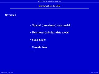
Agenda • Overview of GIS • Introduction to Quantum GIS • Vector Data • Raster Data • Plugins • Fields and Attribution • Creating Data • Map Layout
1. Overview of GIS • Geographic Information System • Wikipedia definition - it is a system designed to capture, store, manipulate, analyze, manage, and present all types of geographically referenced data. • It is used in many applications: Small municipalities, forestry, military, commercial businesses, etc., etc., • What do you do with it?
GIS • Easily measure distances • Easily measure areas • Find overlap between features • Proximity • Everything is related by location. • Tobler's Law
USGS Earthquake Zones http://earthquake.usgs.gov
Outputs from a GIS • Maps • Printed • Digital (PDF, JPEG • Spreadsheets • Databases • Files • Shapefiles • KML
2. Introduction to Quantum GIS • Open Source – It comes with the right to download, run, copy, alter, and redistribute the software. • With source code users have the option • Suggest improvements • Make improvements themselves • Hire a professional to make the changes • Save software from abandonment
Common OS Licensing • Licenses to run in both open and proprietary systems • Apache Software License • BSD (Berkeley Software Distribution) • MIT (Massachusetts Institute of Technology) • License to run in open environments • GPL (General Public License) • LPGL (Lesser General Public License) • MPL (Mozilla Public License)
QGIS • The QGIS project began in February, 2002 • Produced by a Development team • Gary Sherman, Founder • The first release was in July of that year • The first version supported only PostGIS and had no map navigation tools or layer control.
Installing Quantum • http://www.qgis.org • I am going to stick with Windows and Linux Installs. • OSX - http://www.kyngchaos.com/software/qgis • Linux – depending on your distribution of choice you'll have a Debian or RPM install. • Most systems with a large user base have a GIS repository • Ubuntu, Debian, Fedora
Windows • Windows Installer Method • Standalone Installer (recommended for new users) • Installs Quantum (Currently 1.8) • Also installs Current Release of GRASS • Also installs python 2.7 that runs inside of QGIS • Updates uninstall and reinstall the software and save your settings. Must be done manually
Windows Installer cont' • Standalone Method • Geographic Data Abstraction Library • Installs libraries for SID and ECW • SID and ECW are proprietary formats that have special agreements to be used with GDAL • http://www.gdal.org/
OSGEO Install • OSGeo provides an installer that provides everything. • Runs in a “cygwin” type environment • Cygwin provides unix commands and environments on windows machines. • Provides a means to an easy(ier) upgrade path between releases. • Isn't “installed” on your computer.
OSGEO Installer Cont' • Quantum GIS • GDAL • GRASS • OpenEV • And UDIG (a great data viewer).
Toolbars and Panels • Right Click in menu Area • Add Panels • Add Toolbars.
Status Bar • Projection of the QGIS project • Scale • Coordinates
Basic Buttons • Pan • Zoom In • Zoom Out • Pixel Resolution • Zoom to Extent • Zoom to Selection • Zoom to Layer • Zoom to Last Extent • Zoom to Previous Extent • Refresh • Add vector Layer • Add Raster Layer • PostGIS Layer • Spatialite Layer • WMS Layer • New Shapefile Layer • Remove Layer • Oracle Raster Layer • WFS Layer • Hover mouse over them they will pop up a text message telling the user their purpose.
Attribution, Selection, Measurements • Add BookMark • Show Bookmark • Annotation • Identify • Select • Deselect • Attribute Table • Measure • Maptips
Saving a Project • As you are working with QGIS periodically save your datasets. • QGIS creates a .gqs file • XML based • Can be edited in your favorite text editor.
Exercises • Open QGIS • Explore the Toolbars. • Add some data to the Map Display • Use the Identify Features tool to show attribute to some data layers.
Exercise 2 The Exercises are going to be an actual project completed by North River Geographic Systems, Inc in 2009. We are going to cover the Conasauga River Watershed. The watershed is located on the border of Tennessee and Georgia. The data is made up of ESRI Shapefiles. That is the easiest data format to work with for these exercises. 1. If you haven't already, open QGIS. There should be an icon on your desktop or on your start menu (or both). Once QGIS has opened right click with your mouse in the toolbar area. How Many Toolbars are in the Default Installation How many Panels are in the default Installation? Turn off your Managed Layers toolbar. Turn Off your Map Navigation Toolbar. They have disappeared from the interface. Now turn them back on. If you want you can move them from their default location by grabbing the left corner of the toolbar and moving it.
2. Turn your Layers Panel off. Now turn it on by navigating from the View Menu at the top of QGIS 3. Click your Add Vector Data button at the top. Browse to your data folder located under c:\gisdata\QGIStraining\data . Add the CountyBoundaries.shp shapefile to your map. If you do not see any data please be sure to check that you are adding shapefiles.
4. Click your add vector data button at the top and add the subbasin.shp file. You should have something that looks like: 5. Using your identify features tool list all the counties in Georgia and the Counties in Tennessee. In order to identify a feature you must have that layer selected in your layer window. Georgia Tennessee
8. Click on the Subbasin shapefile in your Layers Panel and zoom to the extent of that layer. Note you have several ways to make a selection. 9. Select Whitfield County. Zoom to the extent of the selection. 10. Clear the selection. 11. Save your project in the Exercise 2 Directory! 6. Add the 2010 Urban Areas Shapefile. What is the biggest Urban Area within the CountyBoundaries Shapefile? What are the three biggest Urban Areas that touch/are within the Watershed? 7. Using your navigation tools Zoom to the full extent of all the data layers. You should see something similiar to the graphic below.
3. Adding Vector Data • Supports OGR vector Formats • Shapefiles • KML • CSV • Microstation • MapINFO
Properties • Once Data is added – Right Click and Select Properties • There are different Tabs to help with Vector Data • Style, Label, Fields, General, Metadata, Action Joins, Digrams, Overlay • Style sets the symbology of the Layer. • Symbology can be saved as a qml file
Styles • Set by Fields • Symbolized • Single • Categorized • Graduated • Graduated • Equal Interval, Quantile, Natural Breaks, Standard Deviation, Pretty Breaks
Equal Interval • Equal Interval groups values into equal sized ranges.
Quantile • Each class contains an equal number of features
Natural Breaks • Natural Breaks classes are based on natural groupings of the data.
Standard Deviation • Show Variation from the average value
Pretty Breaks • Data symbolized for non-statisticians
Selecting Vector Data • Selections can be manual
Selecting Vector Data • Selections can be by Attributes • Selections can also be by location (Under Vector Menu - Research)
Exercises • Change the symbology of displayed data • Label features • Add a layer and categorize data by that item.
2. How many main watersheds are located in the Conasauga Watershed. ___________________ BONUS: Why is the Coahulla (pronounced Koa-hull-ahhhh) split into a north and south section? You might need to add more shapefiles to answer this. 3. Label the Watersheds by name on the map display. Rick click on the shapefile layer and select properties. Select the labeling tab. Check "Display Labels". Under Basic Label Options pick Hu_10_Name Exercise Ch 3 It's time to start looking at your data and working with it.. Most of the data you will be working with was downloaded from the Census Bureau, the National Hydro Dataset, and the USDA DataGateway. Some of these datasets were built by me during the course of the CRA project. 1. Add the Watershed.shp file to the Map Display.
5. Change the style of the data layer. Make the polygon fill clear and the outline color orange. 4. Right click on the watershed shapefile and go to properties. Look at the Style tab
5. Change the style of the data layer. Make the polygon fill clear and the outline color orange. 4. Right click on the watershed shapefile and go to properties. Look at the Style tab
6. Save the Style. Right click on the watershed shapefile and click Save Style. Save the file as a .qml file. 7. Once you have saved it remove the watershed shapefile by right clicking on it and selecting remove. Add it again. Right click and select Load Style. Load the qml file you just saved. All of your original settings for this layer have been restored.
8. Select North Coahulla using the select tool. 9. Right click and select “Save Selection As”. You have just saved the North Coahulla section of the watershed. 10. Right click watershed.shp and open the Attribute table. We haven't covered this part yet in the class but it's good to know for the purposes of the exercise. 11. Toggle editing on the attribute layer. The Toggle editing Toolbar is a small icon with a pencil located at the bottom of the Attribute Window.