Exploring Atomic Structure: Wave Nature of Light and Quantum Mechanics
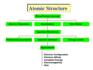
This comprehensive exploration delves into the principles of atomic structure, emphasizing the wave nature of light and its quantized energy through photons. It covers key concepts, including wavelength, frequency, and the speed of light, supported by historical insights such as Planck's discoveries and Einstein's photon theory. The discussion extends to line spectra and the Bohr model, revealing limitations and the foundational principles of quantum mechanics, including Schrödinger’s equation and the properties of orbitals governed by quantum numbers.

Exploring Atomic Structure: Wave Nature of Light and Quantum Mechanics
E N D
Presentation Transcript
The Wave Nature of Light • All waves have a characteristic wavelength, l, and amplitude, A. • Frequency, n, of a wave is the number of cycles which pass a point in one second. • Speed of a wave, c, is given by its frequency multiplied by its wavelength: • For light, speed = c = 3.00x10⁸ m s-1. • A Brief History of Time
Quantized Energy and Photons • Planck: energy can only be absorbed or released from atoms in certain amounts called quanta. • The relationship between energy and frequency is • where h is Planck’s constant ( 6.626 10-34 J s ) .
Quantized Energy and Photons • The Photoelectric Effect and Photons • Einstein assumed that light traveled in energy packets called photons. • The energy of one photon is:
Line Spectra and the Bohr Model • Line Spectra • Radiation composed of only one wavelength is called monochromatic. • Radiation that spans a whole array of different wavelengths is called continuous. • White light can be separated into a continuous spectrum of colors. • Note that there are no dark spots on the continuous spectrum that would correspond to different lines.
Line Spectra and the Bohr Model • Bohr Model • Colors from excited gases arise because electrons move between energy states in the atom. (Electronic Transition)
Line Spectra and the Bohr Model • Bohr Model • Since the energy states are quantized, the light emitted from excited atoms must be quantized and appear as line spectra. • After lots of math, Bohr showed that • where n is the principal quantum number (i.e., n = 1, 2, 3, … and nothing else).
Line Spectra and the Bohr Model • Bohr Model • We can show that • When ni > nf, energy is emitted. • When nf > ni, energy is absorbed
Line Spectra and the Bohr Model Bohr Model Mathcad (Balmer Series) CyberChem (Fireworks) video
Line Spectra and the Bohr Model • Limitations of the Bohr Model • Can only explain the line spectrum of hydrogen adequately. • Can only work for (at least) one electron atoms. • Cannot explain multi-lines with each color. • Electrons are not completely described as small particles. • Electrons can have both wave and particle properties.
The Wave Behavior of Matter • Knowing that light has a particle nature, it seems reasonable to ask if matter has a wave nature. • Using Einstein’s and Planck’s equations, de Broglie showed: • The momentum, mv, is a particle property, whereas is a wave property. • de Broglie summarized the concepts of waves and particles, with noticeable effects if the objects are small.
The Wave Behavior of Matter • The Uncertainty Principle • Heisenberg’s Uncertainty Principle: on the mass scale of atomic particles, we cannot determine exactly the position, direction of motion, and speed simultaneously. • For electrons: we cannot determine their momentum and position simultaneously. • If Dx is the uncertainty in position and Dmv is the uncertainty in momentum, then
Energy and Matter E = m c2
Quantum Mechanics and Atomic Orbitals • Schrödinger proposed an equation that contains both wave and particle terms. • Solving the equation leads to wave functions. • The wave function gives the shape of the electronic orbital. [“Shape” really refers to density of electronic charges.] • The square of the wave function, gives the probability of finding the electron ( electron density ).
Quantum Mechanics and Atomic Orbitals Solving Schrodinger’s Equation gives rise to ‘Orbitals.’ These orbitals provide the electron density distributed about the nucleus. Orbitals are described by quantum numbers.
Quantum Mechanics and Atomic Orbitals • Orbitals and Quantum Numbers • Schrödinger’s equation requires 3 quantum numbers: • Principal Quantum Number, n. This is the same as Bohr’s n. As n becomes larger, the atom becomes larger and the electron is further from the nucleus. ( n = 1 , 2 , 3 , 4 , …. ) • Azimuthal Quantum Number, . This quantum number depends on the value of n. The values of begin at 0 and increase to (n - 1). We usually use letters for (s, p, d and f for = 0, 1, 2, and 3). Usually we refer to the s, p, d and f-orbitals. • Magnetic Quantum Number, m. This quantum number depends on . The magnetic quantum number has integral values between - and + . Magnetic quantum numbers give the 3D orientation of each orbital.
Quantum Mechanics and Atomic Orbitals • Orbitals and Quantum Numbers
Representations of Orbitals The s-Orbitals
Representations of Orbitals The p-Orbitals
Orbitals and Their Energies Orbitals CD Many-Electron Atoms
Many-Electron Atoms Electron Spin and the Pauli Exclusion Principle
Many-Electron Atoms • Electron Spin and the Pauli Exclusion Principle • Since electron spin is quantized, we define ms = spin quantum number = ½. • Pauli’s Exclusions Principle: no two electrons can have the same set of 4 quantum numbers. • Therefore, two electrons in the same orbital must have opposite spins.
Figure 6.27 Orbitals CD Figure 6.27
Orbitals CD Figure 6.28
Orbitals and Their Energies Orbitals CD Many-Electron Atoms
Metals, Nonmetals, and Metalloids Metals Figure 7.14
Periodic Trends • Two Major Factors: • principal quantum number, n, and • the effective nuclear charge, Zeff.
Electron Affinities • Electron affinity is the opposite of ionization energy. • Electron affinity: the energy change when a gaseous atom gains an electron to form a gaseous ion: • Cl(g) + e- Cl-(g) • Electron affinity can either be exothermic (as the above example) or endothermic: • Ar(g) + e- Ar-(g)
Group Trends for the Active Metals Group 1A: The Alkali Metals
Group Trends for the Active Metals Group 2A: The Alkaline Earth Metals
Group Trends for Selected Nonmetals Group 6A: The Oxygen Group
Group Trends for Selected Nonmetals Group 7A: The Halogens
Group Trends for the Active Metals • Group 1A: The Alkali Metals • Alkali metals are all soft. • Chemistry dominated by the loss of their single s electron: • M M+ + e- • Reactivity increases as we move down the group. • Alkali metals react with water to form MOH and hydrogen gas: • 2M(s) + 2H2O(l) 2MOH(aq) + H2(g)
Group Trends for the Active Metals • Group 2A: The Alkaline Earth Metals • Alkaline earth metals are harder and more dense than the alkali metals. • The chemistry is dominated by the loss of two s electrons: • M M2+ + 2e-. • Mg(s) + Cl2(g) MgCl2(s) • 2Mg(s) + O2(g) 2MgO(s) • Be does not react with water. Mg will only react with steam. Ca onwards: • Ca(s) + 2H2O(l) Ca(OH)2(aq) + H2(g)