MULTIPLE TESTING: POWER AND TYPE I ERROR
MULTIPLE TESTING: POWER AND TYPE I ERROR. Andrew Morris Wellcome Trust Centre for Human Genetics March 7, 2003. Outline. Multiple testing. Bonferonni correction. Genome-wide association studies. Randomisation procedures. LOD scores and genome-wide significance levels for linkage.

MULTIPLE TESTING: POWER AND TYPE I ERROR
E N D
Presentation Transcript
MULTIPLE TESTING:POWER AND TYPE I ERROR Andrew Morris Wellcome Trust Centre for Human Genetics March 7, 2003
Outline • Multiple testing. • Bonferonni correction. • Genome-wide association studies. • Randomisation procedures. • LOD scores and genome-wide significance levels for linkage.
Multiple testing: example X X XX X X X X XXX X X X X X X X
Multiple testing: example X X XX X X X X XXX X X X X X X X Significant 5% level
Multiple testing • Significance level α. • Perform N independent tests of null hypothesis. • Number of tests in which null hypothesis is rejected, in samples ascertained from population in which null hypothesis is true, given by binomial distribution, parameters N and α. • Expect to see Nα rejections of null hypothesis by chance.
Example: multiple TDTs • Screen of genomic region for association of disease with 100 SNPs. • Simulate TDT values under null hypothesis of no association: chi-squared distribution with one degree of freedom.
Bonferroni correction • Total number of rejections of null hypothesis over all tests denoted by R. Pr(R>0) = 1-Pr(R=0)= 1-(1-α)N • Need to set α’ = Pr(R>0) to required significance level over all tests. Referred to as the experimentwise error rate. • For TDT example, to achieve overall experimentwise significance level of α’=0.05: 0.05 = 1-(1-α)100 -> α = 0.000513 • Pointwise significance level of 0.05%.
Genome-wide association screens • Risch & Merikangas (1996). • 100,000 genes. • Type 10 SNPs in each gene. • 1 million tests of null hypothesis of no association. • To achieve experimentwise significance level of 5%, require pointwise p-value less than 5.129 x 10⁻⁸.
Bonferroni correction - problems • Assumes each test of the null hypothesis to be independent. • If not true, Bonferroni correction to significance level is conservative. • Loss of power to reject null hypothesis. • Example: genome-wide association screen across linked SNPs – correlation between tests due to LD between loci.
Solutions??? • Focus on candidate genes to reduce the number of tests performed, requiring a less stringent significance level. • Increase power by multi-locus analyses of haplotypes: reduces number of tests. • Publish “near” significant associations and hope they can be replicated in independent studies.
Example: multi-allelic TDT (1) • Original TDT developed for di-allelic marker loci. • Various generalisations to multi-allelic systems: ETDT, GTDT, TDTMAX. • For TDTMAX, calculate TDT statistic for each allele in turn, and use maximum to test null hypothesis of no association between disease and marker.
Example: multi-allelic TDT (2) • Allele 1: • 31 transmissions from heterozygous parents. • 30 non-transmissions from heterozygous parents. TDT1 = (31-30)2/(31+30) = 0.016
Example: multi-allelic TDT (2) • Allele 2: • 54 transmissions from heterozygous parents. • 27 non-transmissions from heterozygous parents. TDT2 = (54-27)2/(54+27) = 9.000
Example: multi-allelic TDT (3) • TDTMAX = 9.000. • p-value assuming chi-squared distribution with one degree of freedom is 0.003. • Five tests performed: Bonferroni corrected experimentwise significance level for overall 1% type I error rate is 0.002. • Cannot reject null hypothesis of no association between disease and marker locus.
Example: multi-allelic TDT (4) • Bonferonni correction conservative since TDTs for multiple alleles at same locus are correlated. • Generate null distribution of TDTMAX statistic by simulation. • Randomisation procedures…
Randomisation procedures • Calculate test statistic XOBS for observed sample of data. • Generate R pseudo-samples of data from observed sample under null hypothesis. • Calculate test statistic Xi for each pseudo-sample. • p-value given by proportion of pseudo-samples for which Xi ≥ XOBS.
Example: multi-allelic TDT (5) • Under null hypothesis of no association between disease and marker locus, alleles are transmitted at random from parents to affected offspring. • Generate pseudo-samples of data by permuting the transmitted and non-transmitted alleles of parents at random. • Calculate TDTMAX statistic for each pseudo sample.
Observed TDT: 9.000 Exceeded 842 times in 100,000 pseudo samples. p-value: 0.00842
Randomisation procedures - problems • Computationally intensive, so may not always be practical – combine permutation procedure and Bonferroni correction. • May not be clear how to simulate from null distribution.
Single locus LOD scores (1) • Results of linkage studies generally presented as LOD scores: LOD = log10[P(D|θ)MAX/P(D|θ=0.5)] • Sample of data is 10LOD times more likely to have been ascertained from population under alternative hypothesis of linkage than the null hypothesis of no linkage. • For single locus analysis, traditionally use LOD score of 3 as threshold for rejecting null hypothesis of no linkage. • Can convert LOD score to chi-squared statistic: X2 = 4.6LOD, so LOD 3 corresponds to pointwise p-value of 0.0001 (1 df test).
Single locus LOD scores (2) • Why so stringent? Does not take account of prior probability of linkage… • Two loci are said to be linked if: • they are on the same chromosome; • they are separated by less than 30Mb. • Depends on total length of the genome (~3300Mb) and relative lengths of chromosomes. • Can be shown that prior probability of linkage is ~0.02.
Single locus LOD scores (3) • Posterior probability of linkage (L) given sample of data (D) calculated by Bayes’ Theorem: P(L|D) = P(D|L)P(L) . P(D|L)P(L)+P(D|NL)P(NL) • It then follows that P(L|D) = Z/(Z+λ), where Z = P(D|L)/P(D|NL) = 10LOD and λ = P(NL)/P(L) is prior odds of no linkage. • For LOD score of 3, Z = 1000. For prior probability of linkage P(L) = 0.02, λ = 49. Thus P(L|D) = 0.95. • Mendelian diseases: can calculate P(D|L) exactly.
LOD scores: genome screen • Search of the genome for evidence of linkage using multiple markers. • Could adjust significance level by Bonferroni correction, but does not take account of the strong correlation between linked markers. • Lander & Kruglyak (1995) propose calculation of genome-wide significance level to allow for multiple testing.
Genome-wide significance level (1) • How often will a LOD score exceed some threshold T by chance in a whole genome screen? • The number of regions R of the genome in which the LOD score exceeds T is given by a Poisson distribution with mean: μ(T) = [C+9.2ρGT]αP(T) where C is the number of chromosomes in the genome, G is the length of the genome (Morgans), αP(T) is the pointwise significance level of T. • The parameter ρ is the crossover rate between genotypes being compared: depends on study design. • Genome-wide significance level: αG(T) = P(R>1) = 1-P(R=0) = 1-exp[-μ(T)] ≈ μ(T).
Genome-wide significance level (2) • Suggestive linkage: statistical evidence expected to occur once at random in genome scan, μ(T)=1. • Significant linkage: statistical evidence expected to occur 0.05 times in genome scan, μ(T) = 0.05. • Highly significant linkage: statistical evidence expected to occur 0.001 times in a genome scan, μ(T) = 0.001.
Genome-wide significance level (4) • Is the genome-wide significance level too stringent: • Study only looked at a few markers? NO: likely that study stopped after first significant linkage – investigator may have continued until entire genome searched if no positive signals identified. • Study involved sparse screen of genome? NO: likely that positive signals will be followed up by higher density searches.
Examples • IDDM • 96 sib pairs: average 10cM spacing. • Followed up regions with LOD > 1, with additional sib pair sets. • Significant linkage at HLA, suggestive linkage on 8q and X, near suggestive linkages on 11q and 6q. • Schizophrenia • Near significant linkages on chromosome 6p in large collection of pedigrees. • Replicated in two independent data sets.
Replication • Linkage and association signals must be replicated in independent studies to be credible. • Replication studies test an established prior hypothesis, so multiple testing problem not an issue. • Failure to replicate does not disprove the linkage or association, unless the power of the replication study is very high. • Competing results of several replication studies may reflect population heterogeneity, diagnostic differences, random sample variation. • Combined analysis or meta analysis…
Summary • Multiple testing inflates the type I error rate of hypothesis test. • Need stringent significance levels. • Bonferroni correction conservative. • Guidelines are available for genome-wide linkage studies. • Replication of results necessary for confirmation.

