On Model Validation Techniques
On Model Validation Techniques. Alex Karagrigoriou University of Cyprus "Quality - Theory and Practice” , ORT Braude College of Engineering, Karmiel , May 2012. OUTLINE. Introduction Graphical Methods Likelihood Method Kolmogorov Test Chi-Squared Tests Tests based on Measures.

On Model Validation Techniques
E N D
Presentation Transcript
On Model Validation Techniques Alex Karagrigoriou University of Cyprus "Quality - Theory and Practice”, ORT Braude College of Engineering, Karmiel, May 2012
OUTLINE • Introduction • Graphical Methods • Likelihood Method • Kolmogorov Test • Chi-Squared Tests • Tests based on Measures
After fitting a distribution model to a data set when performing life data analysis, we are often interested in diagnosing the model's fit or comparing the fit of different distributions. In addition to the engineering knowledge that should always govern the choice of a distribution model, there are many statistical tools that can help in deciding whether or not a distribution model is a good choice from a statistical point of view. These tools can also be used to compare the fit of different distributions.
Reliability Terms • Mean Time To Failure (MTTF) for non-repairable systems • Mean Time Between Failures for repairable systems (MTBF) • Reliability Probability (survival) R(t) • Failure Probability (cumulative density function) F(t)=1-R(t) • Failure Probability Density f(t) • Failure Rate (hazard rate) λ(t) • Mean residual life (MRL)
Exponential Distribution Very commonly used, even in cases to which it does not apply (simple); Applications: Electronics, mechanical components etc. • Normal Distribution Very straightforward and widely used; Applications: Electronics, mechanical components etc. • Lognormal Distribution • Very powerful and can be applied todescribe various failure processes; • Applications: Electronics, material, structure etc. • Weibull Distribution • Very powerful and can be applied to • describe various failure processes; • Applications: Electronics, mechanical • components, material, structure etc. Time Distributions (Models) of the Failure Density
Probability Plots – Graphical Validation Probability plotting (e.g. Q-Q plot) is a graphical method that allows a visual assessment of the model fit. Once the model parameters have been estimated, the probability plot can be created. The next figure shows a comparison of the probability plots of the two choices (Weibulll & Exponential) using the data set.
Problems typical with reliability & survival data Censoring when the observation period ends, not all units have failed - some are survivors) Lack of Failures if there is too much censoring, even though a large number of units may be under observation, the information in the data is limited due to the lack of enough failures) Practical difficulty when planning reliability assessment tests and analyzing failure data.
Type I Censoring – Right Censoring n items are observed during a fixed time period [0, T]. The number of failures r is random. n-r items (also random) will be in operation (censored) at the end of the time period. Also called "right censoring" since the failure times to the right (i.e., larger than T) are missing.
Type II Censoring We run the test until we observe exactly r failures. The time period T is random. n-r units are in operation (nonrandom). In Type II censoring we know in advance how many failure times we have - this helps when planning adequate tests. However, an open-ended random test time is generally impractical from a management point of view and this type of testing is rarely seen.
Readout or Interval Censored Data Sometimes exact times of failure are not known; only an interval of time in which the failure occurred is recorded.
Likelihood Value Use the MLE (Maximum Likelihood Estimation) method to estimate the parameters. Then, the likelihood value can be used to assess the fit: The distribution with the largest L value is the best fit.
Table: Comparing the log-likelihood value for comparing the fit of two distributions. The log-likelihood value for the Weibull distribution is greater than that for the exponential distribution (i.e. the Weibull distribution is statistically a better fit).
Modified Kolmogorov-Smirnov (KS) Test The standard (KS) test is used for continuous distributions with known parameters. The Modified KS test is used when the parameters are unknown and need to be estimated. For N failure times , we define to be the empirical distribution function. The Modified KS test uses the maximum of the absolute difference between and the fitted cumulative distribution function, Q(t):
The distribution of the Modified KS test in the case of the null hypothesis (i.e. data set drawn from the fitted distribution) can be calculated. The test returns the probability that . A high probability value, close to 1, indicates that there is a significant difference between the theoretical distribution and the data set. The value for the Weibull distribution is smaller thus: the Weibull distribution is statistically a better fit.
Chi-Squared Test The chi-squared test relies on the idea of grouping the data into a suitable number of intervals. Grouping involves a loss of information, and there is also often considerable arbitrariness in how the intervals are chosen. The optimal number k of intervals for a sample of size N may be estimated from Sturges' Rule Let Ni be the number of data points in the i interval and ni the expected number according to the fitted distribution. The chi-squared statistic is
A high probability value, close to 1, indicates that there is a significant difference between the theoretical distribution and the data set. Table: Comparing two distributions using the chi-squared test The value for the Weibull distribution is smaller (i.e. the Weibull distribution is statistically a better fit).
Empirical model fitting – Distribution Free • (Kaplan-Meier) approach • No underlying model (Weibull, lognormal etc) is assumed • K-M estimation is an empirical (non-parametric) procedure • Exact times of failure are required
Methods based on Measures Kullback-Leibler: Kagan: Cressie and Read: Matusita: Hellinger: Csiszar:
The BHHJ Power Divergence [Basu et. al (1998)] where (1.5.4) The BHHJ family reduces to the Kullback-Leibler divergenceforα↓0 and to the square of L2 distance for α = 1.
Discrete cases: Distance between 2 binomial/multinomial , (1.5.5)
The AIC Model Selection Criterion For the construction of AIC, Akaike used the K-L measure Akaike proposed the evaluation of the 2nd term (expected LogLik) using minus twice the mean expected LogLik Finally, he provided an unbiased estimator of the expected LogLik:
The AIC Model Selection Criterion where p is the number of unknown parameters involved in the model/distribution. In our case: Weibull model: AIC=2x48.42 + 4=100.84 Exponential : AIC=2x55.04 + 2=112.08 The Weibull fit is better.
Other Model Selection Methods where p is the number of unknown parameters involved in the model/distribution.
The DIC Model Selection The DIC criterion is derived based on the BHHJ measure.
CompareBHHJ testwiththegoodnessoffittestsbasedon theKullbackmeasure (KL), theKaganmeasure (Pearson chi-square test), theMatusitameasure(Mat),and the Cressie and Read measure (CR). • Threedifferentvaluesoftheindex αare used: α = 0.01, 0.05&0.10. • Boththepowerandthetype I errorareinvestigated. • Simulatedresults: A trinomial distribution is used with n=150 and a numberof10000 simulationshavebeencreated.
Goodness of Fit Tests POWER vs ‘SIZE’ of the TEST % of rejections when H1: M(150, 0.2, 0.7, 0.1) holds % of rejections when Ho: M(150, 0.2, 0.6, 0.2) holds