Quantum computing
Quantum computing. COMP308 Lecture notes based on: Introduction to Quantum Computing http://www.cs.uwaterloo.ca/~cleve/CS497-F07 Richard Cleve, Institute for Quantum Computing, University of Waterloo Introduction to Quantum Computing and Quantum Information Theory

Quantum computing
E N D
Presentation Transcript
Quantum computing COMP308 Lecture notes based on: Introduction to Quantum Computing http://www.cs.uwaterloo.ca/~cleve/CS497-F07 Richard Cleve, Institute for Quantum Computing, University of Waterloo Introduction to Quantum Computing and Quantum Information Theory Dan C. Marinescu and Gabriela M. Marinescu Computer Science Department , University of Central Florida
number of transistors 109 108 107 106 105 year 104 1975 1980 1985 1990 1995 2000 2005 Moore’s Law • Measuring a state (e.g. position) disturbs it • Quantum systems sometimes seem to behave as if they are in several states at once • Different evolutions can interfere with each other Following trend … atomic scale in 15-20 years Quantum mechanical effects occur at this scale:
Quantum mechanical effects Additional nuisances to overcome? or New types of behavior to make use of? [Shor ’94]: polynomial-time algorithm for factoring integers on a quantum computer This could be used to break most of the existing public-key cryptosystems, including RSA, and elliptic curve crypto [Bennett, Brassard ’84]: provably secure codes with short keys
quantum information theory classical information theory Also with quantum information: • Faster algorithms for combinatorial search problems • Fast algorithms for simulating quantum mechanics • Communication savings in distributed systems • More efficient notions of “proof systems” Quantum information theory is a generalization of the classical information theory that we all know—which is based on probability theory
What is a quantum computer? • A quantum computer is a machine that performs calculations based on the laws of quantum mechanics, which is the behavior of particles at the sub-atomic level.
Introduction • “I think I can safely say that nobody understands quantum mechanics” - Feynman • 1982 - Feynman proposed the idea of creating machines based on the laws of quantum mechanics instead of the laws of classical physics. • 1985 - David Deutsch developed the quantum turing machine, showing that quantum circuits are universal. • 1994 - Peter Shor came up with a quantum algorithm to factor very large numbers in polynomial time. • 1997 - Lov Grover develops a quantum search algorithm with O(√N) complexity
Representation of Data - Qubits A bit of data is represented by a single atom that is in one of two states denoted by |0> and |1>. A single bit of this form is known as a qubit A physical implementation of a qubit could use the two energy levels of an atom. An excited state representing |1> and a ground state representing |0>. Light pulse of frequency for time interval t Excited State Nucleus Ground State Electron State |0> State |1>
2 1 2 1 2 2 1 2 Representation of Data - Superposition A single qubit can be forced into a superposition of the two states denoted by the addition of the state vectors: |> = |0> + |1> Where and are complex numbers and | | + | | = 1 A qubit in superposition is in both of the states |1> and |0 at the same time
1 1 1 √8 √8 √8 Representation of Data - Superposition Light pulse of frequency for time interval t/2 State |0> State |0> + |1> • Consider a 3 bit qubit register. An equally weighted superposition of all possible states would be denoted by: |> = |000> + |001> + . . . + |111>
One qubit • Mathematical abstraction • Vector in a two dimensional complex vector space (Hilbert space) • Dirac’s notation ket column vector bra row vector bra dual vector (transpose and complex conjugate)
A bit versus a qubit are complex numbers • A bit • Can be in two distinct states, 0 and 1 • A measurement does not affect the state • A qubit • can be in state or in state or in any other state that is a linear combination of the basis state • When we measure the qubit we find it • in state with probability • in state with probability
The Boch sphere representation of one qubit • A qubit in a superposition state is represented as a vector connecting the center of the Bloch sphere with a point on its periphery. • The two probability amplitudes can be expressed using Euler angles.
Two qubits • Represented as vectors in a 2-dimensional Hilbert space with four basis vectors • When we measure a pair of qubits we decide that the system it is in one of four states • with probabilities
Measuring two qubits • Before a measurement the state of the system consisting of two qubits is uncertain (it is given by the previous equation and the corresponding probabilities). • After the measurement the state is certain, it is 00, 01, 10, or 11 like in the case of a classical two bit system.
Measuring two qubits (cont’d) • What if we observe only the first qubit, what conclusions can we draw? • We expect that the system to be left in an uncertain sate, because we did not measure the second qubit that can still be in a continuum of states. The first qubit can be • 0 with probability • 1 with probability
Bell state 1/sqrt(2) |0> + 1/sqrt(2) |1> Measurement of a qubit in that state gives 50% of time logic 0, 50% of time logic. Can also be denoted as |+>
Entanglement • Entanglement is an elegant, almost exact translation of the German term Verschrankung used by Schrodinger who was the first to recognize this quantum effect. • An entangled pair is a single quantum system in a superposition of equally possible states. The entangled state contains no information about the individual particles, only that they are in opposite states. • The important property of an entangled pair is that the measurement of one particle influences the state of the other particle. Einstein called that “Spooky action at a distance".
Operations on Qubits - Reversible Logic • Due to the nature of quantum physics, the destruction of information in a gate will cause heat to be evolved which can destroy the superposition of qubits. Ex. The AND Gate Input Output In these 3 cases, information is being destroyed A C B • This type of gate cannot be used. We must use Quantum Gates.
Quantum Gates • Quantum Gates are similar to classical gates, but do not have a degenerate output. i.e. their original input state can be derived from their output state, uniquely. They must be reversible. • This means that a deterministic computation can be performed on a quantum computer only if it is reversible. Luckily, it has been shown that any deterministic computation can be made reversible.(Charles Bennet, 1973)
One qubit gates • I identity gate; leaves a qubit unchanged. • X or NOT gate transposes the components of an input qubit. • Y gate. • Z gate flips the sign of a qubit. • H the Hadamard gate.
Quantum Gates - Hadamard • Simplest gate involves one qubit and is called a Hadamard Gate (also known as a square-root of NOT gate.) Used to put qubits into superposition. H H State |1> State |0> State |0> + |1> Note: Two Hadamard gates used in succession can be used as a NOT gate
Quantum Gates - Controlled NOT • A gate which operates on two qubits is called a Controlled-NOT (CN) Gate. If the bit on the control line is 1, invert the bit on the target line. Input Output A’ A - Target B’ B - Control Note: The CN gate has a similar behavior to the XOR gate with some extra information to make it reversible.
H Example Operation - Multiplication By 2 • We can build a reversible logic circuit to calculate multiplication by 2 using CN gates arranged in the following manner: Input Output 0 Carry Bit Ones Bit
Quantum Gates - Controlled Controlled NOT (CCN) • A gate which operates on three qubits is called a Controlled Controlled NOT (CCN) Gate. Iff the bits on both of the control lines is 1,then the target bit is inverted. Output Input A’ A - Target B’ B - Control 1 C’ C - Control 2
A Universal Quantum Computer • The CCN gate has been shown to be a universal reversible logic gate as it can be used as a NAND gate. Output Input A’ A - Target B’ B - Control 1 C’ C - Control 2 When our target input is 1, our target output is a result of a NAND of B and C.
Classical and quantum systems Probabilistic states: Quantum states: Diracnotation: |000, |001, |010, …, |111are basis vectors, so
Dirac bra/ket notation Ket:ψalways denotes a column vector, e.g. Convention: Bra:ψalways denotes a row vector that is the conjugate transpose of ψ, e.g. [*1 *2 *d] Bracket:φψ denotes φψ, the inner product of φandψ
Recall conjugate transpose Rotation by : Maps |0 |1 |1 |0 NOT (bit flip): Maps |0 |0 |1 |1 Phase flip: Basic operations on qubits (I) (0) Initialize qubit to |0 or to |1 (1) Apply a unitary operation U(formallyU†U=I ) Examples:
H0 Reflection about this line H1 Basic operations on qubits (II) 1 More examples of unitary operations: (unitary rotation) Hadamard: 0
0+1 Basic operations on qubits (III) 1 ψ1 (3) Apply a “standard” measurement: ψ0 ||2 0 ||2 … and the quantum state collapses to 0 or 1 () There exist other quantum operations, but they can all be “simulated” by the aforementioned types Example: measurement with respect to a different orthonormal basis {ψ0, ψ1}
Distinguishing between two states Let be in state or Question 1: can we distinguish between the two cases? • Distinguishing procedure: • apply H • measure This works because H+=0 andH−=1 Question 2: can we distinguish between 0 and +? Since they’re not orthogonal, they cannot be perfectlydistinguished … but statistical difference is detectable
Unitary operations: Measurements: Operations on n-qubit states (U†U = I) … and the quantum state collapses
Question: what are the states of the individual qubits for 1. ? 2. ? Entanglement Suppose that two qubits are in states: The state of the combined system their tensor product: Answers: 1. 2. ?? ... this is an entangled state
qubits: time U W #1 V #2 #3 #4 unitary operations measurements Structure among subsystems
0 1 1 0 1 1 0 0 1 1 0 1 Quantum circuits Computation is “feasible” if circuit-size scales polynomially
CNOT a two qubit gate • Two inputs • Control • Target • The control qubit is transferred to the output as is. • The target qubit • Unaltered if the control qubit is 0 • Flipped if the control qubit is 1.
Final comments on the CNOT gate • CNOT preserves the control qubit (the first and the second component of the input vector are replicated in the output vector) and flips the target qubit (the third and fourth component of the input vector become the fourth and respectively the third component of the output vector). • The CNOT gate is reversible. The control qubit is replicated at the output and knowing it we can reconstruct the target input qubit.
(do nothing) U The resulting 4x4 matrix is Maps basis states as: 00 0U0 01 0U1 10 1U0 11 1U1 Example of a one-qubit gate applied to a two-qubit system Question: what happens if U is applied to the first qubit?
Controlled-U gates U Resulting 4x4 matrix is controlled-U = Maps basis states as: 00 00 01 01 10 1U0 11 1U1
a a ≡ X b ab H H 0 +1 0−1 H H 0−1 0−1 Controlled-NOT(CNOT) Note: “control” qubit may change on some input states!