Download
1 / 20
200 likes | 354 Vues
A Quick Illustration of JPEG 2000. Presented by Kim-Huei Low Chun Data Fok. Overview. Introduction Approach Illustration Annex B-H Comparison with JPEG Conclusion References Questions. Figure: Picture of Data using JPEG (75% compression ratio, 15KB). Figure:

E N D
A Quick Illustration of JPEG 2000 Presented by Kim-Huei Low Chun Data Fok
Overview • Introduction • Approach • Illustration • Annex B-H • Comparison with JPEG • Conclusion • References • Questions Figure: Picture of Data using JPEG (75% compression ratio, 15KB) Figure: Picture of Kim using J2K (0.5bpp, 3.8KB)
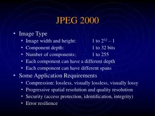
Introduction • JPEG 2000 • Drafted by the international JPEG (Joint Bi-level Image Experts Group) and JBIG (Joint Photographic Experts Group) groups. • Replaces traditional JPEG. • Focuses on hardware implementation. • Our goal • Present a simplified version of the standard. • Give new users a grasp of JPEG 2000.
Approach • Follow the same order as the standard. • Explain the background. • Illustrate each feature. • Discuss its applications. • List the pros and cons. • Will skip Annex A, C and D. • Feature wise, it’s not important. Figure: 0.25bpp J2K Image (11KB); Raw Image’s Size is 1MB
Illustration: Annex B • Tile division • Large images can be broken down into smaller pieces, called tiles. • Tiles are processed independently Figure: Original DWT Figure: Precinct Selection Figure: Sub-band Selection Figure: Code-block Selection
Illustration: Annex B • Progression Order • Layer or Resolution Progressive Figure: 1bpp, 0.5bpp, 0.05bpp and 0.01bpp J2K Image with Layer or Resolution Progression.
Illustration: Annex B • Progression Order • Component Progressive Figure: 1bpp, 0.5bpp, 0.1bpp and 0.01bpp J2K Image with Component Progression.
Illustration: Annex B • Progression Order • Position Progressive Figure: 1bpp, 0.5bpp and 0.1bpp J2K Image with Position Progression.
Illustration: Annex E • Quantization • Reversible vs Irreversible • Target bit rate=0.5 bpp • Step size=1 Figure: Irreversible Explicit Quantization (868B) Figure: Irreversible Implicit Quantization (787B) Figure: Reversible Quantization (16KB)
Illustration: Annex E • Irreversible Explicit Quantization • Target bit rate=0.5 bpp • Different step size Figure: Step Size 1 (868B) Figure: Step Size 0.1 (11.9KB) Figure: Step Size 0.0078 (16.3KB)
Illustration: Annex E • Irreversible Implicit Quantization • Target bit rate=0.5 bpp • Different step size Figure: Step Size 1 (787B) Figure: Step Size 0.1 (11.7KB) Figure: Step Size 0.0078 (16.3KB)
Illustration: Annex F • Discrete Wavelet Transformation (DWT) • Reversible = 5x3 filter (lossless compression) • Irreversible = 9x7 filter (efficient lossy compression)
Illustration: Annex F • Lossless vs Lossy DWT • Different decomposition level • Higher decomposition levels – higher overhead Figure: Lossless, NL=14 (275KB) Figure: Lossy, NL=14 (99KB) Figure: Lossless, NL=3 (274KB) Figure: Lossy, NL=3 (98KB)
Illustration: Annex F • Discard of high frequency sub-bands • High compression, smaller file size • Same quality • Amortize decomposition level overhead • Optimal/Ideal: Encode up to the last visually distinguishable low frequency sub-band Figure: NL=3, 8.3636bpp (274KB) Figure: NL=14, 0.9948bpp (32.6KB)
Illustration: Annex G • DC Level Shifting • Similar to JPEG • New pixel value = Pixel value - 128 • Component Decorrelating Transformation • Reversible vs Irreversible Figure: Raw Image; 0.035bpp J2K Image with RCT; 0.035bpp J2K Image with ICT
Illustration: Annex H • Region of Interest (ROI) Encoding • Efficient use of bit rate • If bit rate is too low, encoding without ROI may look better overall Figure: Raw Image; 0.07bpp J2K Image with ROI; 0.07bpp J2K Image without ROI
Illustration: Comparison of JPEG 2000 with JPEG • 10 test images, 50+ compression ratios • PSNR vs File Size Figure: PSNR Curve
Illustration: Comparison of JPEG 2000 with JPEG • Much smaller files • Much better quality Figure: 0.08bpp J2K Image (8KB); 0.1563bpp JPEG Image (16KB);
Conclusion • Excellent compression rate • Fully exploits the advantage of DWT • Capable of handling extremely large images • Lots of user-selectable features • Efficient for hardware implementation • Most advanced image compression standard • Implication of MPEG 2000?
References • International Telecommunication Union (ITU), International Organization for Standardization (ISO), “JPEG 2000 Implementation in Java,” http://jpeg2000.epfl.ch, October 16th, 2003. • ISO/IEC JTCI/SC29 WGI, JPEG 2000 Editor Martin Boliek, Charilaos Christopoulos, Eric Majani, “JPEG 2000 Image Coding System,” http://www.jpeg.org/CDs15444.html, March 16th, 2000.