Functional Enrichment Analysis :
Introduction to Systems Biology 2012. Functional Enrichment Analysis :. making sense of big data. Aaron Brooks & Fang Yin Lo 8/21/2012. Insight. Experimental Design. Data analysis. Data collection. Mischel et al, 2004. From knots to knowledge. What is functional enrichment?

Functional Enrichment Analysis :
E N D
Presentation Transcript
Introduction to Systems Biology 2012 Functional Enrichment Analysis: making sense of big data Aaron Brooks & Fang Yin Lo 8/21/2012
Insight Experimental Design Data analysis Data collection Mischel et al, 2004
From knots to knowledge • What is functional enrichment? - Tools and caveats (e.g. DAVID and pvals) • How can you apply these tools to large, complex analysis problems (i.e. automation)?
Why functional enrichment analysis? Interesting glioblastoma study Gene Function Common Pathways Gene Gene Gene Gene Gene Gene e.g. Glycolysis Common Functions Draw 6 marbles (k) e.g. sugar metabolism Urn problem: How likely am I to draw 3 or more marbles? • N: population size • m: # of positives in the population • k: # of draws • q: # of positives Total: 15 marbles (N): 5 red (m) 10 black (N-m)
The workflow of typical enrichment tools e.g. Gene Ontology (GO), KEGG Pathway, etc e.g. GO Terms that are enriched in the input gene list Nucleic Acids Research, 2009, Vol. 37, No. 1 1–13
(the database for annotation, visualization and integrated discovery) • Diverse, web-based functional analysis tool • Integrates a suite of databases and statistical tools (GO, KEGG, Interpro, Disease) • User-friendly, • Problematic for large analysis problems (many independent sets) staRt your engines http://baliga.systemsbiology.net/events/sysbio/content/bicluster-307 http://baliga.systemsbiology.net/events/sysbio/content/bicluster-353
What if you had many sets to analyze? AUTOMATION!!!
topGO • An R package that facilitates semi-automated enrichment analysis for Gene Ontology • Three main Steps: • Prepare data -create a topGO object with list of genes identiers, gene-to-GO annotations) • Run enrichment tests • Display theresults
Structured controlled vocabularies (ontologies) that describe relationships between gene products and their associated biological roles cellular components : the parts of a cell or its extracellular environment molecular functions: activities, such as catalytic or binding activities, that occur at the molecular level (e.g. catalytic activity, Toll receptor binding) biological processes: series of events accomplished by one or more ordered assemblies of molecular functions (e.g. signal transduction, pyrimidine metabolic process )
GO structure • Directed Acyclic Graph(DAG) • Child terms are more specialized • Child can havemore than one parent
Data preparation # Install topGO and Affymetrix Human Genome U133 Plus 2.0 Array annotation data > source("http://bioconductor.org/biocLite.R") > biocLite("topGO") > biocLite("hgu133plus2.db") > geneSets # Input a list a genes #Boot the gaggle > library(gaggle) > gaggleInit() #load the library > library(topGO) > library(hgu133plus2.db)
Data preparation ### Initializing the analysis ### # hgu133plus2ACCNUM: an R object that contains mappings between the manufacturers identifiers and gene names of Affymetrix Human Genome U133 Plus 2.0 Array # all.genes: all background genes ( gene universe ) > all.genes <- ls(hgu133plus2ACCNUM)
Other annotation packages at Bioconductor Other annotation packages can be found at: http://www.bioconductor.org/packages/release/data/annotation/
Data preparation: Input gene lists • ### Make gene lists ### • # We will make a list that includes two sets of genes of interest • # Initialize the list: • >glioblastoma.genes = list() • http://baliga.systemsbiology.net/events/sysbio/content/bicluster-307 • # broadcast 'bicluster 307 genes' to R • >glioblastoma.genes[["bc307"]] = sapply(getNameList(),tolower) • Do the same for the other gene list: • http://baliga.systemsbiology.net/events/sysbio/content/bicluster-353 • >glioblastoma.genes[["bc353"]] = sapply(getNameList(),tolower)
Data preparation: make topGO object • ## Analyze genes in bc353 first • > relevant.genes <- factor(as.integer(all.genes %in% glioblastoma.genes[["bc353"]])) • > names(relevant.genes) <- all.genes • # Construct the topGOdata object for automated analysis • >GOdata.BP <- new("topGOdata", ontology='BP', allGenes = relevant.genes, annotationFun = annFUN.db, affyLib = 'hgu133plus2.db') # ontology:'BP','MF; or 'CC' # allGenes: named vector of type numeric or factor. The names attribute contains the genes identifiers. The genes listed in this object define the gene universe. # annotationFun: function that maps gene identifiers to GO terms. # annFUN.db extracts the gene-to-GO mappings from the affyLib object # affyLib: character string containing the name of the Bioconductorannotaion package for a specific microarray chip.
Run Enrichment Analysis • > results <- runTest(GOdata.BP, algorithm = 'classic', statistic = 'fisher’)
Analysis of results: summary # generate a summary of the enrichment analysis > results.table <- GenTable(GOdata.BP, results, topNodes = length(results@score)) • # How many GO terms were tested? • > dim(results.table)[1] • # reduce results to GO terms passing Benjamini-Hochberg multiple hypothesis corrected pval <= 0.05, FDR <= 5% • >results.table.bh <- results.table[which(p.adjust(results.table[,"result1"],method="BH")<=0.05),]
Analysis of results: get significant GO terms • # reduce results to GO terms passing Benjamini-Hochberg multiple hypothesis corrected pval <= 0.05, FDR <= 5% • >results.table.bh <- results.table[which(p.adjust(results.table[,"result1"],method="BH")<=0.05),] • # How many terms are enriched? • >dim(results.table.bh)[1] • # What are the top ten terms? • >results.table.bh[1:10,]
Analysis of results: get genes in top GO terms • # Get all the genes annotated to a specific GO term of interest: • >GOid.of.interest = results.table.bh[1,"GO.ID"] • >all.term.genes = genesInTerm(GOdata.BP,GOid.of.interest)[[1]] • # Which of these genes is in the bicluster? • >genes.of.interest <- intersect(glioblastoma.genes[["bc353"]],all.term.genes) • # print table with probe ID and gene symbol • >gene.symbol= toTable(hgu133plus2SYMBOL[genes.of.interest]) • # print table with probe ID and gene names • >gene.name= toTable(hgu133plus2GENENAME[genes.of.interest]) • # Combine the information of the genes, output to csvfile: • >cbind(gene.symbol,gene.name[,2]) • >write.csv(cbind(gene.symbol,gene.name[,2]), file = "glioblastoma.genes_bc353_in_immune response.csv“)
Automation results <- list() for( bc in names(glioblastoma.genes) ) { cat(paste("Computing functional enrichment for...",bc,"\n")) relevant.genes <- factor(as.integer(all.genes %in% glioblastoma.genes[[bc]])) names(relevant.genes) <- all.genes GOdata.BP <- new("topGOdata", ontology='BP', allGenes = relevant.genes, annotationFun = annFUN.db, affyLib = 'hgu133plus2.db') results[[bc]] <- GenTable(GOdata.BP,runTest(GOdata.BP, algorithm = 'classic', statistic = 'fisher'),topNodes = length(results@score)) }
Other algorithms supported by topGO • Standard implementations of GO testing compute the significance of a node independent of the significance of the neighboring nodes (‘classic’) • Other algorithms take into considerations of the GO structure and try to find more specific GO terms (e.g.’elim’, ‘weight’,‘weight01’,etc) Alexa et al. (2006). Bioinformatics (2006) 22 (13): 1600-1607.
Other algorithms supported by topGO # Try running other algorithms and compare the results: >r1.BP.elim = runTest(GOdata.BP, algorithm = 'elim', statistic = 'fisher') >r1.BP.weight = runTest(GOdata.BP, algorithm = 'weight', statistic = 'fisher‘) # This will take a while… # After the runs are done, visually compare resulting p values from different algorithms: >pValue.classic <- score(r1.BP) >pValue.elim <- score(r1.BP.elim)[names(pValue.classic)] >pValue.weight <- score(r1.BP.weight)[names(pValue.classic)] >gstat <- termStat(GOdata.BP, names(pValue.classic)) >gSize <- gstat$Annotated / max(gstat$Annotated) * 4 >colMap <- function(x) { .col <- rep(rev(heat.colors(length(unique(x)))), time = table(x)) return(.col[match(1:length(x), order(x))]) } >gCol <- colMap(gstat$Significant) >plot(pValue.classic, pValue.elim, xlab = "p-value classic", ylab = "p-value elim",pch = 19, cex = gSize, col = gCol)
Broadcasting gene list to DAVID 4. Broadcast to DAVID 1. In R: > broadcast(geneSetGenes) 2. 3. Select target: DAVID
Broadcasting gene list to DAVID Gene list and population background being analyzed Clustering options and contingency A group of terms having similar biological meaning due to sharing similar gene members Original database/resources where the terms orient Enriched terms associate with input gene list Modified Fisher Exact p-values Corrected p-values
Some remaining challenges Realistically positioning the role of enrichment P-values in the current data-mining environment: • high-throughput enrichment data-mining environment is extremely complicated • Variations of the user gene list size • deviation of the number of genes associated with each annotation • gene overlap between annotation • incompleteness of annotation content • strong connectivity/dependency among genes • unbalanced distributions of annotation content Limitation of multiple testing correction on enrichment P-values • common multiple testing correction techniques maybe overly conservative approaches if there are thousands or even more annotation terms involved in the analysis • Genome Inform. 2005;16:106-115.; Nucleic Acids Research, 2009, Vol. 37, No. 1 1–13 Cross-comparing enrichment analysis results derived from multiple gene lists • the size of the gene list impacts the absolute enrichment P-values, therefore • difficult to directly compare the absolute enrichment P-values across gene lists
Some remaining challenges some may treat the resulting enrichment P-values as a scoring system that plays a advisory role more of an exploratory procedure, with the aid of enrichment P-value, rather than a pure statistical solution. the specificity of enrichment analysis is more impacted by non-statistical layers than it is by statistical methods alone Nat. Protoc. 2008. doi: 10.1038/nprot.2008.211 Nucleic Acids Research, 2009, Vol. 37, No. 1 1–13
Working with topGO data object # work with Godata.BP # obtaining all genes > a = genes(GOdata.BP) > str(a) chr [1:31777] "1007_s_at" "1053_at" "117_at" "121_at" "1255_g_at" "1294_at" ... # number of genes > numGenes(GOdata.BP) [1] 31777 # The list of significant genes can be accessed using the method sigGenes() > sg = sigGenes(GOdata.BP) > str(sg) chr [1:22] "201291_s_at" "202095_s_at" "202589_at" "202705_at" "203213_at" ...
Working with topGO data object # accessing information related to GO and its structure # which GO terms are available for analysis: > ug = usedGO(GOdata.BP) > str(ug) chr [1:10921] "GO:0000002" "GO:0000003" "GO:0000012" "GO:0000018" "GO:0000019" ... # select some random GO terms: (1). count the number of annotated genes and (2) obtain their annotation > sel.terms <- sample(usedGO(GOdata.BP), 10) > sel.terms [1] "GO:0032913" "GO:0043372" "GO:0044259" "GO:0032700" "GO:0043122" "GO:2001141" "GO:0060587" [8] "GO:0071352" "GO:0007256" "GO:0051343“ # Check what are the genes annotated to a specific GO term: > genesInTerm(GOdata.BP, "GO:0032913" ) $`GO:0032913` [1] "208650_s_at" "208651_x_at" "209771_x_at" "209772_s_at" "216379_x_at" "266_s_at" # Number of genes annotated to the selected GO terms: > num.ann.genes <- countGenesInTerm(GOdata.BP, sel.terms) > num.ann.genes GO:0032913 GO:0043372 GO:0044259 GO:0032700 GO:0043122 GO:2001141 GO:0060587 GO:0071352 GO:0007256 6 36 111 12 454 6809 2 5 11 GO:0051343 2
Working with topGO data object > ann.genes <- genesInTerm(GOdata.BP, sel.terms) > str(ann.genes) List of 10 $ GO:0032913: chr [1:6] "208650_s_at" "208651_x_at" "209771_x_at" "209772_s_at" ... $ GO:0043372: chr [1:36] "1554519_at" "1555689_at" "1565358_at" "1569748_at" ... $ GO:0044259: chr [1:111] "1554383_a_at" "1555540_at" "1555896_a_at" "1556499_s_at" ... $ GO:0032700: chr [1:12] "1552798_a_at" "1556190_s_at" "201300_s_at" "207160_at" ... $ GO:0043122: chr [1:454] "1552360_a_at" "1552703_s_at" "1552798_a_at" "1552804_a_at" ... $ GO:2001141: chr [1:6809] "121_at" "1316_at" "1405_i_at" "1487_at" ... $ GO:0060587: chr [1:2] "201525_at" "207092_at" $ GO:0071352: chr [1:5] "201940_at" "201941_at" "201942_s_at" "201943_s_at" ... $ GO:0007256: chr [1:11] "1558984_at" "203652_at" "206362_x_at" "207347_at" ... $ GO:0051343: chr [1:2] "207514_s_at" "214286_at"
Analysis of results: get genes in top GO terms • #We can also look at multiple GO terms at the same time: • > GOids.of.interest = results.table.bh[c(1:10),"GO.ID"] • > all.term.genes = genesInTerm(GOdata.BP,GOids.of.interest) • # Which of these genes is in the bicluster? • > genes.of.interest <- sapply(names(all.term.genes),function(x){intersect(all.term.genes[[x]],glioblastoma.genes[["bc353"]])}) • # print table with probe ID and gene symbol: • > geneSynmol.of.interest <- lapply(names(genes.of.interest),function(x){toTable(hgu133plus2SYMBOL[genes.of.interest[[x]]])}) • > names(geneSynmol.of.interest)<- GOids.of.interest