Jeff Edmonds York University

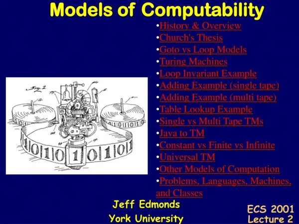
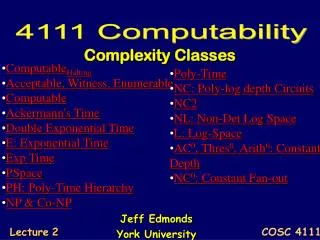
1. 4111 Computability Complexity Classes ComputableHalting Acceptable, Witness, Enumerable Computable Ackermann's Time Double Exponential Time E: Exponential Time Exp Time PSpace PH: Poly-Time Hierarchy NP & Co-NP Poly-Time NC: Poly-log depth Circuits NC2 NL: Non-Det Log Space L: Log-Space AC0, Thres0, Arith0: Constant Depth NC0: Constant Fan-out Jeff Edmonds York University Lecture2 COSC 4111

2. Complexity Classes Computable Exp Poly A complexity class is a set of computational problems that have a similar difficulty in computing them. Design a new class: • Choose some model • Java or Circuits • Deterministic or Nondeterministic • Limit some resource • Time or Space • to Log, Poly, Exp, …. Co-NP NP

3. Complexity Classes Computable Exp Poly A complexity class is a set of computational problems that have a similar difficulty in computing them. We will start with a small weak class and work our way up. Each will be a super set of the previous Proving C1 C2 is not too hard. • Prove C2can simulate C1. Proving C1 C2 is hard. • Prove P ϵC2and P ϵ C1. Co-NP NP (unless pointed out)

4. Complexity Classes Computable Exp complete Poly A complexity class is a set of computational problems that have a similar difficulty in computing them. A problem is complete for a class if being able to solve this problem fast means that you can solve every problem in the class fast. Co-NP NP

5. NC0 x43 x25 x31 constant AND AND OR OR NOT constant OR NC0 = Set of computational problems computed by circuits of and/or/not gates each with two inputs of constant depth. • Each output bit can only depend ona constant number of the input bits. • But can compute any function of these bits. NC is short for “Nick’s Class” after Nick Pippenger

6. NC0 NC0 = Set of computational problems computed by circuits of and/or/not gates each with two inputs of constant depth. • Eg: It can compute the next configuration of a TM.

7. AC0 x1 ¬x2 x3 …¬xn ¬x1 x2 ¬x3 … xn x1 x2 ¬x3 … ¬xn AND AND AND … OR AC0 = Set of computational problems computed by circuits of and/or/not gates each arbitrary fan-in of constant depth and poly-size. = circuits of and/or/not gates each with two inputs any depth but constant # of alternations between and & or. • Arbitrary fan-in means can depend on all the input bits. constant AC is short for “Alternations Class”

8. AC0 x1 ¬x2 x3 …¬xn ¬x1 x2 ¬x3 … xn x1 x2 ¬x3 … ¬xn AND AND AND … OR AC0 = Set of computational problems computed by circuits of and/or/not gates each arbitrary fan-in of constant depth and poly-size. • Depth 2 and 2n size can compute any function but this needs poly-size. • It can’t compute the parity of the input bits because this requires log n alternations of and & or. • Parity is needed for counting & adding. constant

9. Threshold0(Neural Net) x1 x2 x3 … xn w1 w2 w3 … wn Threshold T y y = 1 iff Σi wi×xi ≥ T Threshold0 = Set of computational problems computed by circuits of threshold gates each arbitrary fan-in of constant depth and poly-size. • Early AI used them to build neural net with a constant number of hidden levels. • Theoreticians say they are more powerful than and/or/not, but they still can’t compute parity. • But they do manage to predict if your credit card is stolen. constant

10. Arithmetic0 constant Arithmetic0 = Set of computational problems computed by circuits of +, -, ×, /, =,and≤gates each arbitrary fan-in of constant depth and poly-size real value on each wire. • What you can do on a calculator with a constant number of key strokes. x43 x25 x51 + × + constant constant - × /

11. NC1 x1 x2 xn all AND AND OR OR NOT O(logn) OR NC1 = Set of computational problems computed by circuits of and/or/not gates each with two inputs of constant O(logn) depth. • Each output bit can depend on all input bits. • Can add, multiply, divide, … … NCk allows depth O((logn)k)

12. Log-Space L = Set of computational problems computed by a TM with a read-only tape for the input and a O(log(n)) cell work tape. • clog(n) cells  2clog(n) = ncconfigurations  at most nc time or cycles forever. • Often used for to represent low level computation • Producing inputs for reductions • Producing the nth uniform circuits. TM n x3 x4 xn x1 x2 … q O(log(n)) 0 1 1 0

13. Log-Space L = Set of computational problems computed by a TM with a read-only tape for the input and a O(log(n)) cell work tape. • Can compute everything in NC1. • Do depth first search • Remember the values along the path to the root. TM n x3 x4 xn x1 x2 … q O(log(n)) 0 1 1 0

14. Log-Space L = Set of computational problems computed by a TM with a read-only tape for the input and a O(log(n)) cell work tape. • Can compute every regular language, eg 0*1* • Read input once • Remember which state the Finite State Automata is in. • Actually only O(1) space is needed. TM n x3 x4 xn x1 x2 … q O(1) O(log(n)) 0 1 1 0

15. Log-Space L = Set of computational problems computed by a TM with a read-only tape for the input and a O(log(n)) cell work tape. • Can solve undirected st-connectivity • Use log(n) bits to remember location of “pebble” • Walk the pebble “randomly” from s looking for t. s t

16. Log-Space L = Set of computational problems computed by a TM with a read-only tape for the input and a O(log(n)) cell work tape. • Likely cannot solve directed st-connectivity • Constant number of “pebbles” get stuck. • This requires O(log2(n)) space s t

17. Non-Deterministic Log-Space NL = Set of computational problems computed by a non-deterministic TM with a read-only tape for the input and a O(log(n)) cell work tape. • Fairy Godmother tells you which step to take if possible to get to an accepting computation. TM n x3 x4 xn x1 x2 … q O(log(n)) 0 1 1 0

18. Non-Deterministic Log-Space NL = Set of computational problems computed by a non-deterministic TM with a read-only tape for the input and a O(log(n)) cell work tape. • Can solve directed st-connectivity • Use log(n) bits to remember location of “pebble” • Fairy Godmother tells you which edge to take if possible to get to t. (NL-complete) s t

19. Non-Deterministic Log-Space NL = Set of computational problems computed by a non-deterministic TM with a read-only tape for the input and a O(log(n)) cell work tape. • Directed st-connectivity is complete for NL. • If I can do directed st-connectivity fast •  I can do all problems PNL fast.

20. NL Complete P(I) is true or not Directed graph G BUILD:Oracle for P GIVEN:Oracle for directed st-conn Yes, there is a path in Gfrom s to t or not. PNL  Non-Det Log-Space TM MP computes P  I can compute P fast using this fast algorithm for directed st-connectivity. I

21. NL Complete Directed graph G = BUILD:Oracle for P GIVEN:Oracle for directed st-conn PNL  Non-Det Log-Space TM MP computes P  I can compute P fast using this fast algorithm for directed st-connectivity. I • Nodes are the configs of MP • At most clogn cells  at most 2clogn = ncconfigs  at most 2clogn = ncnodes

22. NL Complete Directed graph G = BUILD:Oracle for P GIVEN:Oracle for directed st-conn PNL  Non-Det Log-Space TM MP computes P  I can compute P fast using this fast algorithm for directed st-connectivity. I • Nodes are the configs of MP • Directed edge <u,v> MP could transition from u to v • Because non-deterministic, out degree ≥ 1

23. NL Complete P(I) is true or not Directed graph G = BUILD:Oracle for P GIVEN:Oracle for directed st-conn Yes, there is a path in Gfrom s to t or not. PNL  Non-Det Log-Space TM MP computes P  I can compute P fast using this fast algorithm for directed st-connectivity. I • Nodes are the configs of MP • Directed edge <u,v> MP could transition from u to v • s is the start configuration of M on I • t is the accepting configuration

24. Non-Deterministic Log-Space NL = Set of computational problems computed by a non-deterministic TM with a read-only tape for the input and a O(log(n)) cell work tape. • Directed st-connectivity is complete for NL. • If I can do directed st-connectivity fast •  I can do all problems PNL fast.

25. Non-Deterministic Log-Space NL = Set of computational problems computed by a non-deterministic TM with a read-only tape for the input and a O(log(n)) cell work tape. • Much more surprisingly (and harder to prove), can solve directed non-st-connectivity • Fairy Godmother tells you a witness to prove that there is no st-path. s t

26. Non-Deterministic Co-Non-Deterministic Deterministic Generally, these classes are different.

27. Co-Non-Deterministic Log Space Non-Deterministic = Log Space Deterministic Here they are the same!

28. NC2 x1 x2 xn AND AND OR OR NOT O((logn)2) OR NC2 = Set of computational problems computed by circuits of and/or/not gates each with two inputs of constant O((logn)2) depth and poly-size. • As a graduate student I helped on a papertrying to prove NC1< NC2. (Obvious but very hard to prove) … NCk allows depth O((logn)k)

29. NC2 x1 x2 xn AND AND OR OR NOT O((logn)2) OR NC2 = Set of computational problems computed by circuits of and/or/not gates each with two inputs of constant O((logn)2) depth and poly-size. • Can solve directed st-connectivity • Can solve everything in NL. (NL-complete) … NCk allows depth O((logn)k)

30. NC2 NC2 = Set of computational problems computed by circuits of and/or/not gates each with two inputs of constant O((logn)2) depth and poly-size. • Can solve directed st-connectivity • Each round <u,v>&<v,w>  <u,w> (transitive closure) n different v’ … <u,v’> <v’,w> <u,v> <v,w> u v w AND AND O(logn) OR <u,w>

31. NC2 NC2 = Set of computational problems computed by circuits of and/or/not gates each with two inputs of constant O((logn)2) depth and poly-size. • Can solve directed st-connectivity • Each round <u,v>&<v,w>  <u,w> (transitive closure) s These were added too. • log(n) rounds • Each round takeslog(n) depth. • Total (logn)2depth s and t are connected. t

32. NC x1 x2 xn AND AND OR OR NOT O((logn)O(1)) OR NC = Set of computational problems computed by circuits of and/or/not gates each with two inputs of constant O((logn)O(1)) depth and poly-size. • What can be done quickly in parallel. …

33. Linear Time Time(O(n)) = Set of computational problems computed by a TM in time O(n). • Time to solve problem ~ Time to read the instance. • Can add two n-bit numbers. • (Does not contain NC, because NC need not be linear sized.) TM n … x3 x4 xn x1 x2 … … q

34. Sorting Time Time(O(nlogn)) = Set of computational problems computed by a TM in time O(nlogn). • Can Sort • Can multiply two n-bit numbers. TM n … x3 x4 xn x1 x2 … … q

35. nc Time Time(O(nc)) = Set of computational problems computed by a TM in time O(nc). TM n … x3 x4 xn x1 x2 … … q

36. Poly-Time P = Set of computational problems computed by a TM in time nO(1). • Considered to be a reasonable algorithm. TM n … x3 x4 xn x1 x2 … … q

37. Non-Deterministic Poly-Time NP = Set of computational problems computed by a non-deterministic TM in time nO(1). • Yes instances have poly-sized witnesses S that verify they are yes instances. No instances do not. • The witness can be found in exponential time • But verified in polynomial time. • Considered to be a unreasonable algorithm. |S| ≤ |I|c Non-Det TM n … x3 x4 xn x1 x2 … … q

38. Non-Deterministic Poly-Time NP complete NP = Set of computational problems computed by a non-deterministic TM in time nO(1). • Yes instances have poly-sized witnesses S that verify they are yes instances. No instances do not. • Eg: Given a circuit, does it have a satisfying assignment |S| ≤ |I|c SAT Poly

39. Non-Deterministic Poly-Time NP complete NP = Set of computational problems computed by a non-deterministic TM in time nO(1). • Formal definition: • Prob  NP iff  poly time Valid • such that Prob(I) =  S Valid(I,S) |S| ≤ |I|c SAT Poly

40. Co-Non-Deterministic Poly-Time CoNP NP not SAT complete complete Co-NP = Set of computational problems whose complement are in NP. Prob(I) = S Valid(I,S) Prob(I) = S Valid(I,S) SAT Poly

41. Poly-Time Hierarchy |S| ≤ |I|c • Ex: Is there an n-character Java program J that solves Sat on all n-bit instances C J C [X=J(C) & C(X) = 1] or [0=J(C) & X C(X) = 0] 2P = 2P = S S’ Valid(I,S,S’) S S’ Valid(I,S,S’) 1P = 1P =

42. Poly-Time Hierarchy 3P = 3P = S S’ S’’ Valid(I,S,S’,S’’) S S’S’’ Valid(I,S,S’,S’’) 2P = 2P =

43. Poly-Time Hierarchy • Ex: Is there a winning n-move strategy for chess in which my moves are S1, S3, …, Sn-1 and my opponent's moves are S2, S4, …, Sn? PH = nP = S1 S2S3 …. Sn-1Sn Valid(I,S1,S2,S3,…,Sn-1,Sn) 3P = 3P =

44. Polynomial-Space PSpace = Set of computational problems computed by a TM with nO(1) cells of work tape. • nO(1) cells  2n configurations  at most 2ntime or cycles forever.  Exponential Time. O(1) O(1) TM nO(1) x3 x4 xn x1 x2 … q

45. Polynomial-Space PSpace = Set of computational problems computed by a TM with nO(1) cell of work tape. • Can compute everything in PH= S1 S2S3 …. Sn-1Sn Valid(I,S1,S2,S3,…,Sn-1,Sn) TM nO(1) x3 x4 xn x1 x2 … q

46. Polynomial-Space PSpace = Set of computational problems computed by a TM with nO(1) cell of work tape. • Can solve most problems about games. • Can understand most things about the game Chess, by studying every way of arranging the pieces. (one such way can be stored in memory.) TM nO(1) x3 x4 xn x1 x2 … q

47. Exp-Time Exp-Time = Set of computational problems computed by a TM in time 2O(n). • Can solve most famous problems in NP, because their witnesses have size cn and hence there are at most 2cn of them. But (likely) can’t solve all of them TM n … x3 x4 xn x1 x2 … … q

48. Exponential-Time E = Set of computational problems computed by a TM in time 2n. • Can solve all problems in NP, because their witnesses have size nc and hence there are at most 2n of them. • In fact, as said, can solve all problems in PSpace. O(1) c TM n … x3 x4 xn x1 x2 … … q

49. Double Exponential-Time Double Exponential-Time = Set of computational problems computed by a TM in time 22. nO(1) TM n … x3 x4 xn x1 x2 … … q

50. Ackermann’s Time Ackermann(5)-Time = Set of computational problems computed by a TM in time Ackermann(5). • But this is only constant time O(1). TM n … x3 x4 xn x1 x2 … … q