Download
1 / 222
2.22k likes | 2.32k Vues
Delve into the fascinating history of computability from Euclid's algorithm for GCD to modern marvels like the Jacquard loom, Babbage's Analytical Engine, and the first transistorized computer. Explore the development of models of computation, including Turing machines and Java programs, in understanding the limits and power of mechanical computation. Discover Church's Thesis, which posits the equivalence of reasonable models of computation and the computability of computational problems. Unravel the evolution of computing, from vacuum tubes to integrated circuits, and ponder the question of what tasks are computable by different models of computation.

E N D
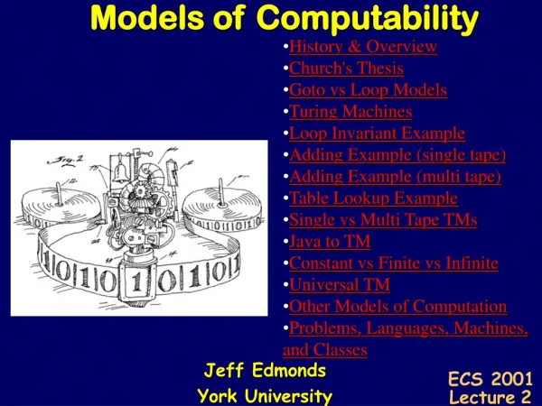
Models of Computability • History & Overview • Church's Thesis • Gotovs Loop Models • Turing Machines • Loop Invariant Example • Adding Example (single tape) • Adding Example (multi tape) • Table Lookup Example • Single vs Multi Tape TMs • Java to TM • Constant vs Finite vs Infinite • Universal TM • Other Models of Computation • Problems, Languages, Machines, and Classes Jeff Edmonds York University • ECS 2001 Lecture2
Please feel free • to ask questions! • Please give me feedbackso that I can better serve you. • Thanks for the feedback that you have given me already.
History of Computability • Euclid said, • “ Let there be an algorithm for GCD” • <y,x mod y> • <x,y> • And so it was. • GCD(a,b) = GCD(x,y) • Euclid (300 BC) • In the beginning: • And it was good. • He gave a new understanding of • “Algorithm”
History of Computability • Unknown • Known • As one gets closer to God, • everything is possible. • We must only learn how to do it. • Euclid (300 BC) • GCD
History of Computability • The Jacquard loom (1801) was one of the first programmable devices. • Weaves complex patterns in textiles. • Controlled by punched cards • This portrait of Jacquard was woven in silk on a Jacquard loom and required 24,000 punched cards to create (1839).
History of Computability • Charles Babbage’s Analytical Engine (1837) • Memory • An arithmetical unit, • Conditional branching and loops, • Making it the first Turing-complete general-purpose computer.
History of Computability • The 1890 census compiled by machine that sorted punched cards. • Reduced required time from eight to one year • Population of 62,947,714
History of Computability • Hilbert • Can every problem be computed? • Or are some Uncomputable? • One of his 23 influential open problems (1900) • Need to formally define • “Algorithm”
History of Computability • A problem is Computable • if it can be computed by a Turing Machine. (1936) • Turing • Halting • Problem • TMComputable • Need to formally define • “Algorithm”
History of Computability • A problem is Computable • if it can be computed by a Turing Machine. (1936) • Turing • Halting • Problem • TMComputable • Though not intended to be practical,the Turing Machine hugely helped • develop and understand the power and limits of mechanical computation.
History of Computability • Vacuum tubes made electronic computing possible • Colossus (1943) 2,400 tubes, ENIAC (1946) 17,000 tubes • 5,000 characters per second • $500,000 ($6 million with inflation). • Helped breaking German codes • Tube failure (every two days, 15 min to locate) • First “bug” was a moth in a tube. • (with Turing)
History of Computability • The first transistorised computer (1953) • Integrated circuits (1968) • Intel 4004 Microprocessors (1971)
Church’s Thesis • Turing • TMComputable • Java • Computable • RecursiveComputable • Are these definitionsequivalent? • Church says “Yes” • All reasonable models of computation are equivalent • as far as what they can compute. • And within a polynomial in time • (except for Quantum Machines) • Need to formally define • “Algorithm”
Church’s Thesis • A Computational Problem Pstates • for each possible input I • what the required output P(I) is. • A Language L is • a computational problem where • the required output is yes/no • An Algorithm/Program/Machine Mis • a set of instructions • for solving a given computational problem P • on a given input I • A Model of Computation is • What is a legal algorithm/program/machine Eg: Sorting Eg: Is the input sorted? Eg: Merge Sort Eg: Java
Church’s Thesis • A Model of Computation (What is a legal Algorithm/Machine/Program) • How the algorithm is specified by finite description. • What defines the current state of the machine. • Eg, how information computed so far is stored. • What line of code it is on or state it is in. • What are the legal operations? Should be a “reasonable” mechanical task. • How the input/output are specified. • Question: Which computational problems are computable by a given model of computation?
Church’s Thesis • Model of Computation: Java • An algorithm/program is specified by Java code. • The current state of the machine is specified by the values of all the variables & data structuresand by which is the next line of code to be executed. • The legal operations are the legal Java commands. • Input/output are read and written to a file.
Church’s Thesis • A computational problem is computable • by a Java Program • by a Turing Machine • by a (simple) Recursive Program • by a (simple) Register Machine • by a Circuit: And/Or/Not, Computer, Arithmetic, & Neural Nets. • by a Non-Deterministic Machine • by a Quantum Machine • by a Context Sensitive Grammar
Church’s Thesis Proof • A computational problem is computable • by a Java Program • by a Turing Machine If a boy can do it, a girl can do it better. If a Java program can do it, Turing Machine can simulate it.
Goto vs Loop Models • Loop Model: • In the early 80’s, structuredprogramming was enforced. • “Goto”s were not allowed. • Programs were controlled withwhile (and if) commands. • Goto Model: • In the 70’s, programs were controlled withgoto (and if) commands. x = 0 print(“Hi”) x = x+1 if( x<10 ) goto line 1 halt 0: 1: 2: 3: 4: for( x = 0; x<10; ++x ) print(“Hi”) Called spaghetti code because computation flow can go all over the place. How many “Hi”s get printed?
Goto vs Loop Models • Loop Model: • In the early 80’s, structuredprogramming was enforced. • “Goto”s were not allowed. • Programs were controlled withwhile (and if) commands. • Goto Model: • In the 70’s, programs were controlled withgoto (and if) commands. x = 0 print(“Hi”) x = x+1 if( x<10 ) goto line 1 halt 0: 1: 2: 3: 4: for( x = 0; x<10; ++x ) print(“Hi”) Called spaghetti code because computation flow can go all over the place. How many “Hi”s get printed?
Goto vs Loop Models • Loop Model: • In the early 80’s, structuredprogramming was enforced. • “Goto”s were not allowed. • Programs were controlled withwhile (and if) commands. • Goto Model: • In the 70’s, programs were controlled withgoto (and if) commands. x = 0 print(“Hi”) x = x+1 if( x<10 ) goto line 1 halt 0: 1: 2: 3: 4: for( x = 0; x<10; ++x ) print(“Hi”) Do these two models have the same power? Can they compute the same things?
Goto vs Loop Models Loop Model: Goto Model: Do these two models have the same power? Can they compute the same things?
Goto vs Loop Models We design a goto program that simulates it. Given an arbitrary loop program: x = 0 print(“Hi”) x = x+1 if( x<10 ) goto line 1 0: 1: 2: 3: for( x = 0; x<10; ++x ) print(“Hi”) Pretty straight forward to replace each loop with a goto.
Goto vs Loop Models Given an arbitrary goto program: We design a loop program that simulates it. Have one big loop that iterates once per line of the goto program. … x = 0 … goto line 18 … halt 11: 38: 99: Loop Invariantt: At each iteration each program has all the same variable values. The loop program has a variable line that specifieswhich line of code the goto program is on.
Goto vs Loop Models Given an arbitrary goto program: We design a loop program that simulates it. line = 1 while( line -1 ) • if( line = 11 ) • x = 0 • ++line … x = 0 … goto line 18 … halt 11: 38: 99: • if( line = 38 ) • line = 18 • if( line = 99 ) • line = -1 end while
Goto vs Loop Models • Loop Model: • In the early 80’s, structuredprogramming was enforced. • “Goto”s were not allowed. • Programs were controlled withwhile (and if) commands. • Goto Model: • In the 70’s, programs were controlled withgoto (and if) commands. x = 0 print(“Hi”) x = x+1 if( x<10 ) goto line 1 halt 0: 1: 2: 3: 4: for( x = 0; x<10; ++x ) print(“Hi”) Hence these do have the same power
Goto vs Loop Models • Loop Model: • In the early 80’s, structuredprogramming was enforced. • “Goto”s were not allowed. • Programs were controlled withwhile (and if) commands. • Loop Invariant Model: • In the 90’s, the importance ofloop invariants was realized. for( x = 0; x<10; ++x ) print(“Hi”) It is still hard for me to know how many “Hi”s get printed
Goto vs Loop Models • Establishing Loop Invariant • <preCond> • codeA • <loop-invariant> • Loop Invariant Model: • In the 90’s, the importance ofloop invariants was realized. • x = 0 • loop • % Loop Inv: x = # “Hi”s printed so far. • exit when x=10 • print(“Hi”) • x = x+1 • end loop • % Post Cond: # “Hi”s get printed is 10. Focus on sequence of states instead of sequence of commands!
Goto vs Loop Models • Maintaining Loop Invariant • <loop-invariant> • ¬<exit Cond> • codeB • <loop-invariant> • Exit • Loop Invariant Model: • In the 90’s, the importance ofloop invariants was realized. • x = 0 • loop • % Loop Inv: x = # “Hi”s printed so far. • exit when x=10 • print(“Hi”) • x = x+1 • end loop • % Post Cond: # “Hi”s get printed is 10.
Goto vs Loop Models • Exit • Clean up loose ends • <loop-invariant> • <exit Cond> • codeC • <postCond> • Loop Invariant Model: • In the 90’s, the importance ofloop invariants was realized. • x = 0 • loop • % Loop Inv: x = # “Hi”s printed so far. • exit when x=10 • print(“Hi”) • x = x+1 • end loop • % Post Cond: # “Hi”s get printed is 10.
Goto vs Loop Models • Loop Invariant Model: • In the 90’s, the importance ofloop invariants was realized. • x = 0 • loop • % Loop Inv: x = # “Hi”s printed so far. • exit when x=10 • print(“Hi”) • x = x+1 • end loop • % Post Cond: # “Hi”s get printed is 10. Proves that IF the program terminates then it works <PreCond>&<code>Þ <PostCond>
Machine Code vs Java • Java Model: • fancy data structures • loops • recursions • object oriented • Machine Model: • one line of code
Machine Code vs Java • Java Model: • fancy data structures • loops • recursions • object oriented • Machine Model: • one line of code • one line of memory cells.
Machine Code vs Java • Java Model: • fancy data structures • loops • recursions • object oriented • Machine Model: • one line of code • one line of memory cells. by Java Program • If a computational problem is computable by a Machine Code • Proof: • Easy simulation
Machine Code vs Java • Java Model: • fancy data structures • loops • recursions • object oriented • Machine Model: • one line of code • one line of memory cells. • If a computational problem is computable by a Machine Code by Java Program • Proof: • This is what a compiler does. • We will prove this after covering Context Free Grammars
TM Model of Computation • A Turing Machine (1936) is the simplest model of computation. • Motivations: • Define the first general model of computation (Previous machines/models did specific predefined tasks.)
TM Model of Computation • A Turing Machine (1936) is the simplest model of computation. • Motivations: • Show that a machine/algorithm does not need a huge set of complex operation but can itself be very simple. • Somehow the power of computation is an “emergent property” • Defn: In philosophy, systems theory, science, and art, emergence is the way complex properties and patterns arise out of a multiplicity of relatively simple interactions.
TM Model of Computation • Computable • A Turing Machine (1936) is the simplest model of computation. • Halting • Problem • Motivations: • Formally define what a legal computation is • so that he could prove that the Halting problem can’t be computed.
TM Model of Computation • A Turing Machine (1936) is the simplest model of computation. • Motivations: • Just as Euclid/Gödelwanted the simplest set of axioms from which to define truth of all mathematical statements, • Turingwanted the simplest set of operations from which to define all algorithms. • Giving multiplication away for free would have felt like cheating.
TM Model of Computation • A Turing Machine (1936) is the simplest model of computation. • Motivations: • It is cool that such a simple model of computation computes everything computable.
TM Model of Computation • A Turing Machine (1936) is the simplest model of computation. • Motivations: • Though not intended to be practical, the Turing Machine hugely helped develop and understand the power and limits of mechanical computation.
TM Model of Computation Model of Computation: Turing Machine • The current configuration of the machine is specified by • The contents of tape • Each cell contains either a zero, one, or blank. (or characters from some other finite alphabet ) • Tape is infinite in one direction • But after a finite number of cells, all are blanks. • Initially the input 101 is presented as b101bb… • As is the output.
TM Model of Computation Model of Computation: Turing Machine q • The current configuration of the machine is specified by • The contents of tape • The current state q • One of some fixed number • One of which is the start state • And one of which is the halting state
TM Model of Computation Model of Computation: Turing Machine q • The current configuration of the machine is specified by • The contents of tape • The current state • The current location of the head. • The machine can move this head left or right. • But does not “know” its current location. • It only knows the value of this current cell.
TM Model of Computation Model of Computation: Turing Machine q q’ • The legal operations are: • Given the current state q • And value c of the cell with the head • The TM looks up in a preset table • The next state q’ • Whether to write a new value to the current cell • Whether to move the head one cell to the right or left • ie Transition function δ(q,c) = <q’,c’,direction>
TM Model of Computation Model of Computation: Turing Machine cϵ∑ seen on tape This is a TM. Nothing more. Nothing less. It gives instructions for “computing” It is abstract. It is NOT practical. We will try to give it “meaning”. Instead of trying to design TMs, we will compile any Java like program into a TM. Current State Transition function δ(q,c) = <q’,c’,direction>
Time • contents of tape • current state • Simple rules like these • produce complex patterns. • TM step: • Current state & cell content at headdetermines which rule to use giving: • how cell contents changes • how head moves • how state changes Tape Cells
Time • contents of tape • current state • Simple rules like these • produce complex patterns. • TM step: • Current state & cell content at headdetermines which rule to use giving: • how cell contents changes • how head moves • how state changes Tape Cells
Time Simple rules like these produce complex patterns. But any meaning has to be added by us. Tape Cells